NCAR JupyterHub Large Data Example Notebook
Note: If you do not have access to the NCAR machine, please look at the AWS-LENS example notebook instead.
This notebook demonstrates how to compare large datasets on glade with ldcpy. In particular, we will look at data from CESM-LENS1 project (http://www.cesm.ucar.edu/projects/community-projects/LENS/data-sets.html). In doing so, we will start a DASK client from Jupyter. This notebook is meant to be run on NCAR’s JupyterHub (https://jupyterhub.hpc.ucar.edu). We will use a subset of the CESM-LENS1 data on glade is located in /glade/p/cisl/asap/ldcpy_sample_data/lens.
We assume that you have a copy of the ldcpy code on NCAR’s glade filesystem, obtained via: git clone https://github.com/NCAR/ldcpy.git
When you launch your NCAR JupyterHub session, you will need to indicate a machine and then you will need your charge account. You can then launch the session and navigate to this notebook.
NCAR’s JupyterHub documentation: https://www2.cisl.ucar.edu/resources/jupyterhub-ncar
Here’s another good resource for using NCAR’s JupyterHub: https://ncar-hackathons.github.io/jupyterlab-tutorial/jhub.html)
You need to run your notebook with the “cmip6-201910” kernel (choose from the dropdown in the upper left.)
Note that the compressed data that we are using was generated for this paper:
Allison H. Baker, Dorit M. Hammerling, Sheri A. Mickelson, Haiying Xu, Martin B. Stolpe, Phillipe Naveau, Ben Sanderson, Imme Ebert-Uphoff, Savini Samarasinghe, Francesco De Simone, Francesco Carbone, Christian N. Gencarelli, John M. Dennis, Jennifer E. Kay, and Peter Lindstrom, “Evaluating Lossy Data Compression on Climate Simulation Data within a Large Ensemble.” Geoscientific Model Development, 9, pp. 4381-4403, 2016 (https://gmd.copernicus.org/articles/9/4381/2016/)
Setup
Let’s set up our environment. First, make sure that you are using the cmip6-2019.10 kernel. Then you will need to modify the path below to indicate where you have cloned ldcpy. (Note: soon we will install ldcpy on Cheyenne/Casper in the cmpi6-2019.10 kernel .)
If you want to use the dask dashboard, then the dask.config link must be set below (modify for your path in your browser).
[1]:
# Make sure you are using the cmpi6-2019.10 kernel

# Add ldcpy root to system path (MODIFY FOR YOUR LDCPY CODE LOCATION)
import sys

sys.path.insert(0, '/glade/u/home/apinard/newldcpy/ldcpy')
import ldcpy

# Display output of plots directly in Notebook
%matplotlib inline
# Automatically reload module if it is editted
%reload_ext autoreload
%autoreload 2

# silence warnings
import warnings

warnings.filterwarnings("ignore")


# if you want to use the DASK daskboard, then modify the below and run
import dask

# dask.config.set(
#    {'distributed.dashboard.link': 'https://jupyterhub.hpc.ucar.edu/ch/user/abaker/proxy/{port}/status'}
# )
[1]:
<dask.config.set at 0x2b3585fb93d0>
Connect to DASK distributed cluster :
(The cluster object is for a single compute node: https://jobqueue.dask.org/en/latest/howitworks.html)
[1]:
from dask_jobqueue import PBSCluster

# For Casper
cluster = PBSCluster(
    queue="casper",
    walltime="02:00:00",
    project="NIOW0001",
    memory="40GB",
    resource_spec="select=1:ncpus=4:mem=40GB",
    cores=4,
    processes=1,
)

# for Cheyenne
# cluster = PBSCluster(
#    queue="regular",
#    walltime="02:00:00",
#    project="NIOW0001",
#    memory="109GB",
#    resource_spec="select=1:ncpus=9:mem=109GB",
#    cores=36,
#    processes=9,
# )


# scale as needed
cluster.adapt(minimum_jobs=1, maximum_jobs=30)
cluster
The scheduler creates a normal-looking job script that it can submit multiple times to the queue:
[3]:
# Look at the job script (optional)
print(cluster.job_script())
#!/usr/bin/env bash

#PBS -N dask-worker
#PBS -q regular
#PBS -A NIOW0001
#PBS -l select=1:ncpus=9:mem=109GB
#PBS -l walltime=02:00:00

/ncar/usr/jupyterhub/envs/cmip6-201910/bin/python -m distributed.cli.dask_worker tcp://10.148.10.15:38275 --nthreads 4 --nprocs 9 --memory-limit 12.11GB --name dummy-name --nanny --death-timeout 60 --interface ib0 --protocol tcp://
[4]:
from dask.distributed import Client

# Connect client to the remote dask workers
client = Client(cluster)
client
[4]:
Client
|
Cluster
|
Note: click on the daskboard link above to see your DASK tasks
The sample data on the glade filesystem
In /glade/p/cisl/asap/ldcpy_sample_data/lens on glade, we have TS (surface temperature), PRECT (precipiation rate), and PS (surface pressure) data from CESM-LENS1. These all all 2D variables. TS and PRECT have daily output, and PS has monthly output. We have the compressed and original versions of all these variables that we would like to compare with ldcpy.
First we list what is in this directory (two subdirectories):
[5]:
# list directory contents
import os

os.listdir("/glade/p/cisl/asap/ldcpy_sample_data/lens")
[5]:
['README.txt', 'lossy', 'orig']
Now we look at the contents of each subdirectory. We have 14 files in each, consisting of 2 different timeseries files for each variable (1920-2005 and 2006-2080).
[6]:
# list lossy directory contents (files that have been lossy compressed and reconstructed)
lossy_files = os.listdir("/glade/p/cisl/asap/ldcpy_sample_data/lens/lossy")
lossy_files
[6]:
['c.FLUT.daily.20060101-20801231.nc',
 'c.CCN3.monthly.192001-200512.nc',
 'c.FLNS.monthly.192001-200512.nc',
 'c.LHFLX.daily.20060101-20801231.nc',
 'c.TS.daily.19200101-20051231.nc',
 'c.SHFLX.daily.20060101-20801231.nc',
 'c.U.monthly.200601-208012.nc',
 'c.TREFHT.monthly.192001-200512.nc',
 'c.LHFLX.daily.19200101-20051231.nc',
 'c.TMQ.monthly.192001-200512.nc',
 'c.PRECT.daily.20060101-20801231.nc',
 'c.PS.monthly.200601-208012.nc',
 'c.Z500.daily.20060101-20801231.nc',
 'c.FLNS.monthly.200601-208012.nc',
 'c.Q.monthly.192001-200512.nc',
 'c.U.monthly.192001-200512.nc',
 'c.CLOUD.monthly.192001-200512.nc',
 'c.so4_a2_SRF.daily.20060101-20801231.nc',
 'c.PRECT.daily.19200101-20051231.nc',
 'c.TAUX.daily.20060101-20801231.nc',
 'c.CLOUD.monthly.200601-208012.nc',
 'c.TS.daily.20060101-20801231.nc',
 'c.FSNTOA.daily.20060101-20801231.nc',
 'c.Q.monthly.200601-208012.nc',
 'c.CCN3.monthly.200601-208012.nc',
 'c.TREFHT.monthly.200601-208012.nc',
 'c.TMQ.monthly.200601-208012.nc',
 'c.PS.monthly.192001-200512.nc']
[7]:
# list orig (i.e., uncompressed) directory contents
orig_files = os.listdir("/glade/p/cisl/asap/ldcpy_sample_data/lens/orig")
orig_files
[7]:
['CLOUD.monthly.200601-208012.nc',
 'LHFLX.daily.20060101-20801231.nc',
 'so4_a2_SRF.daily.20060101-20801231.nc',
 'PRECT.daily.20060101-20801231.nc',
 'TMQ.monthly.192001-200512.nc',
 'TAUX.daily.20060101-20801231.nc',
 'CCN3.monthly.200601-208012.nc',
 'PS.monthly.192001-200512.nc',
 'FLUT.daily.20060101-20801231.nc',
 'PRECT.daily.19200101-20051231.nc',
 'TS.daily.20060101-20801231.nc',
 'PS.monthly.200601-208012.nc',
 'TS.daily.19200101-20051231.nc',
 'Z500.daily.20060101-20801231.nc',
 'SHFLX.daily.20060101-20801231.nc',
 'Q.monthly.200601-208012.nc',
 'TMQ.monthly.200601-208012.nc',
 'U.monthly.200601-208012.nc',
 'FSNTOA.daily.20060101-20801231.nc',
 'TREFHT.monthly.200601-208012.nc',
 'FLNS.monthly.192001-200512.nc',
 'FLNS.monthly.200601-208012.nc']
We can look at how big these files are…
[8]:
print("Original files")
for f in orig_files:
    print(
        f,
        " ",
        os.stat("/glade/p/cisl/asap/ldcpy_sample_data/lens/orig/" + f).st_size / 1e9,
        "GB",
    )
Original files
CLOUD.monthly.200601-208012.nc   3.291160567 GB
LHFLX.daily.20060101-20801231.nc   4.804299285 GB
so4_a2_SRF.daily.20060101-20801231.nc   4.755841518 GB
PRECT.daily.20060101-20801231.nc   4.909326733 GB
TMQ.monthly.192001-200512.nc   0.160075734 GB
TAUX.daily.20060101-20801231.nc   4.856588097 GB
CCN3.monthly.200601-208012.nc   4.053932835 GB
PS.monthly.192001-200512.nc   0.12766304 GB
FLUT.daily.20060101-20801231.nc   4.091392046 GB
PRECT.daily.19200101-20051231.nc   5.629442994 GB
TS.daily.20060101-20801231.nc   3.435295036 GB
PS.monthly.200601-208012.nc   0.111186435 GB
TS.daily.19200101-20051231.nc   3.962086636 GB
Z500.daily.20060101-20801231.nc   3.244290942 GB
SHFLX.daily.20060101-20801231.nc   4.852980899 GB
Q.monthly.200601-208012.nc   3.809397495 GB
TMQ.monthly.200601-208012.nc   0.139301278 GB
U.monthly.200601-208012.nc   4.252600112 GB
FSNTOA.daily.20060101-20801231.nc   4.101201335 GB
TREFHT.monthly.200601-208012.nc   0.110713886 GB
FLNS.monthly.192001-200512.nc   0.170014618 GB
FLNS.monthly.200601-208012.nc   0.148417532 GB
Open datasets
First, let’s look at the original and reconstructed files for the monthly surface Pressure (PS) data for 1920-2006. We begin by using ldcpy.open_dataset() to open the files of interest into our dataset collection. Usually we want chunks to be 100-150MB, but this is machine and app dependent.
[9]:
# load the first 86 years of montly surface pressure into a collection

col_PS = ldcpy.open_datasets(
    "cam-fv",
    ["PS"],
    [
        "/glade/p/cisl/asap/ldcpy_sample_data/lens/orig/PS.monthly.192001-200512.nc",
        "/glade/p/cisl/asap/ldcpy_sample_data/lens/lossy/c.PS.monthly.192001-200512.nc",
    ],
    ["orig", "lossy"],
    chunks={"time": 500},
)
col_PS
dataset size in GB 0.46
[9]:
<xarray.Dataset>
Dimensions:     (collection: 2, lat: 192, lon: 288, time: 1032)
Coordinates:
  * lat         (lat) float64 -90.0 -89.06 -88.12 -87.17 ... 88.12 89.06 90.0
  * lon         (lon) float64 0.0 1.25 2.5 3.75 5.0 ... 355.0 356.2 357.5 358.8
  * time        (time) object 1920-02-01 00:00:00 ... 2006-01-01 00:00:00
    cell_area   (lat, collection, lon) float64 dask.array<chunksize=(192, 1, 288), meta=np.ndarray>
  * collection  (collection) <U5 'orig' 'lossy'
Data variables:
    PS          (collection, time, lat, lon) float32 dask.array<chunksize=(1, 500, 192, 288), meta=np.ndarray>
Attributes:
    Conventions:      CF-1.0
    source:           CAM
    case:             b.e11.B20TRC5CNBDRD.f09_g16.031
    title:            UNSET
    logname:          mickelso
    host:             ys0219
    Version:          $Name$
    revision_Id:      $Id$
    initial_file:     b.e11.B20TRC5CNBDRD.f09_g16.001.cam.i.1920-01-01-00000.nc
    topography_file:  /glade/p/cesmdata/cseg/inputdata/atm/cam/topo/USGS-gtop...
    history:          Tue Nov  3 13:51:10 2020: ncks -L 5 PS.monthly.192001-2...
    NCO:              netCDF Operators version 4.7.9 (Homepage = http://nco.s...
    cell_measures:    area: cell_area
data_type: cam-fv- collection: 2
- lat: 192
- lon: 288
- time: 1032
- lat(lat)float64-90.0 -89.06 -88.12 ... 89.06 90.0
- long_name :
- latitude
- units :
- degrees_north
array([-90. , -89.057592, -88.115183, -87.172775, -86.230366, -85.287958, -84.34555 , -83.403141, -82.460733, -81.518325, -80.575916, -79.633508, -78.691099, -77.748691, -76.806283, -75.863874, -74.921466, -73.979058, -73.036649, -72.094241, -71.151832, -70.209424, -69.267016, -68.324607, -67.382199, -66.439791, -65.497382, -64.554974, -63.612565, -62.670157, -61.727749, -60.78534 , -59.842932, -58.900524, -57.958115, -57.015707, -56.073298, -55.13089 , -54.188482, -53.246073, -52.303665, -51.361257, -50.418848, -49.47644 , -48.534031, -47.591623, -46.649215, -45.706806, -44.764398, -43.82199 , -42.879581, -41.937173, -40.994764, -40.052356, -39.109948, -38.167539, -37.225131, -36.282723, -35.340314, -34.397906, -33.455497, -32.513089, -31.570681, -30.628272, -29.685864, -28.743455, -27.801047, -26.858639, -25.91623 , -24.973822, -24.031414, -23.089005, -22.146597, -21.204188, -20.26178 , -19.319372, -18.376963, -17.434555, -16.492147, -15.549738, -14.60733 , -13.664921, -12.722513, -11.780105, -10.837696, -9.895288, -8.95288 , -8.010471, -7.068063, -6.125654, -5.183246, -4.240838, -3.298429, -2.356021, -1.413613, -0.471204, 0.471204, 1.413613, 2.356021, 3.298429, 4.240838, 5.183246, 6.125654, 7.068063, 8.010471, 8.95288 , 9.895288, 10.837696, 11.780105, 12.722513, 13.664921, 14.60733 , 15.549738, 16.492147, 17.434555, 18.376963, 19.319372, 20.26178 , 21.204188, 22.146597, 23.089005, 24.031414, 24.973822, 25.91623 , 26.858639, 27.801047, 28.743455, 29.685864, 30.628272, 31.570681, 32.513089, 33.455497, 34.397906, 35.340314, 36.282723, 37.225131, 38.167539, 39.109948, 40.052356, 40.994764, 41.937173, 42.879581, 43.82199 , 44.764398, 45.706806, 46.649215, 47.591623, 48.534031, 49.47644 , 50.418848, 51.361257, 52.303665, 53.246073, 54.188482, 55.13089 , 56.073298, 57.015707, 57.958115, 58.900524, 59.842932, 60.78534 , 61.727749, 62.670157, 63.612565, 64.554974, 65.497382, 66.439791, 67.382199, 68.324607, 69.267016, 70.209424, 71.151832, 72.094241, 73.036649, 73.979058, 74.921466, 75.863874, 76.806283, 77.748691, 78.691099, 79.633508, 80.575916, 81.518325, 82.460733, 83.403141, 84.34555 , 85.287958, 86.230366, 87.172775, 88.115183, 89.057592, 90. ]) - lon(lon)float640.0 1.25 2.5 ... 356.2 357.5 358.8
- long_name :
- longitude
- units :
- degrees_east
array([ 0. , 1.25, 2.5 , ..., 356.25, 357.5 , 358.75])
- time(time)object1920-02-01 00:00:00 ... 2006-01-...
- long_name :
- time
- bounds :
- time_bnds
array([cftime.DatetimeNoLeap(1920, 2, 1, 0, 0, 0, 0), cftime.DatetimeNoLeap(1920, 3, 1, 0, 0, 0, 0), cftime.DatetimeNoLeap(1920, 4, 1, 0, 0, 0, 0), ..., cftime.DatetimeNoLeap(2005, 11, 1, 0, 0, 0, 0), cftime.DatetimeNoLeap(2005, 12, 1, 0, 0, 0, 0), cftime.DatetimeNoLeap(2006, 1, 1, 0, 0, 0, 0)], dtype=object) - cell_area(lat, collection, lon)float64dask.array<chunksize=(192, 1, 288), meta=np.ndarray>
- long_name :
- gauss weights
Array Chunk Bytes 884.74 kB 442.37 kB Shape (192, 2, 288) (192, 1, 288) Count 12 Tasks 2 Chunks Type float64 numpy.ndarray - collection(collection)<U5'orig' 'lossy'
array(['orig', 'lossy'], dtype='<U5')
- PS(collection, time, lat, lon)float32dask.array<chunksize=(1, 500, 192, 288), meta=np.ndarray>
- units :
- Pa
- long_name :
- Surface pressure
- cell_methods :
- time: mean
Array Chunk Bytes 456.52 MB 110.59 MB Shape (2, 1032, 192, 288) (1, 500, 192, 288) Count 20 Tasks 6 Chunks Type float32 numpy.ndarray
- Conventions :
- CF-1.0
- source :
- CAM
- case :
- b.e11.B20TRC5CNBDRD.f09_g16.031
- title :
- UNSET
- logname :
- mickelso
- host :
- ys0219
- Version :
- $Name$
- revision_Id :
- $Id$
- initial_file :
- b.e11.B20TRC5CNBDRD.f09_g16.001.cam.i.1920-01-01-00000.nc
- topography_file :
- /glade/p/cesmdata/cseg/inputdata/atm/cam/topo/USGS-gtopo30_0.9x1.25_remap_c051027.nc
- history :
- Tue Nov 3 13:51:10 2020: ncks -L 5 PS.monthly.192001-200512.nc newPS.nc
- NCO :
- netCDF Operators version 4.7.9 (Homepage = http://nco.sf.net, Code = http://github.com/nco/nco)
- cell_measures :
- area: cell_area
- data_type :
- cam-fv
Data comparison
Now we use the ldcpy package features to compare the data.
Surface Pressure
Let’s look at the comparison statistics at the first timeslice for PS.
[10]:
ps0 = col_PS.isel(time=0)
ldcpy.compare_stats(ps0, "PS", ["orig", "lossy"])
| orig | lossy | |
|---|---|---|
| mean | 96750 | 96734 |
| variance | 8.4254e+07 | 8.4249e+07 |
| standard deviation | 9179.1 | 9178.8 |
| min value | 1.0299e+05 | 1.0298e+05 |
| max value | 51967 | 51952 |
| probability positive | 1 | 1 |
| number of zeros | 0 | 0 |
| lossy | |
|---|---|
| max abs diff | 31.992 |
| min abs diff | 0 |
| mean abs diff | 15.806 |
| mean squared diff | 249.83 |
| root mean squared diff | 18.303 |
| normalized root mean squared diff | 0.0003587 |
| normalized max pointwise error | 0.00062698 |
| pearson correlation coefficient | 1 |
| ks p-value | 1.6583e-05 |
| spatial relative error(% > 0.0001) | 69.085 |
| max spatial relative error | 0.00048247 |
| Data SSIM | 0.91512 |
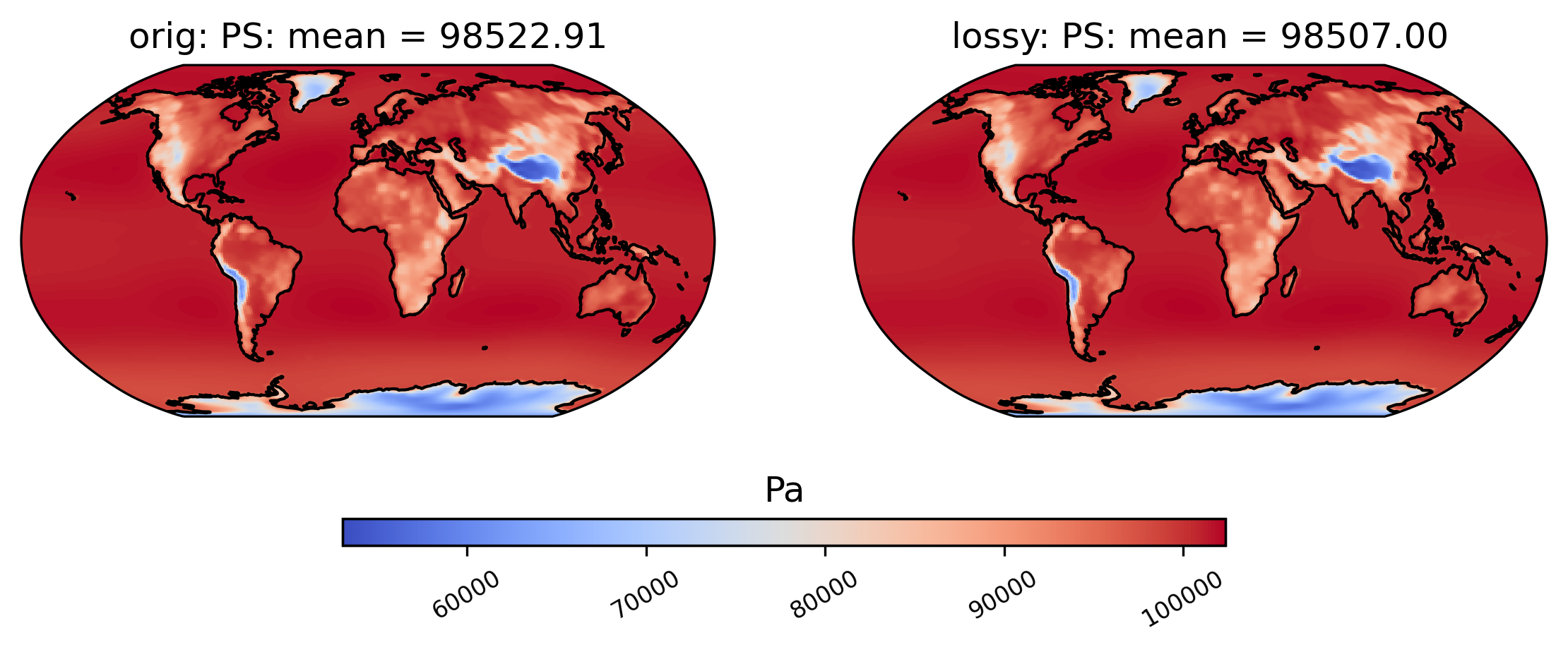
Now we make a plot to compare the mean PS values across time in the orig and lossy datasets.
[11]:
# comparison between mean PS values (over the 86 years) in col_PS orig and lossy datasets
ldcpy.plot(col_PS, "PS", sets=["orig", "lossy"], calc="mean")
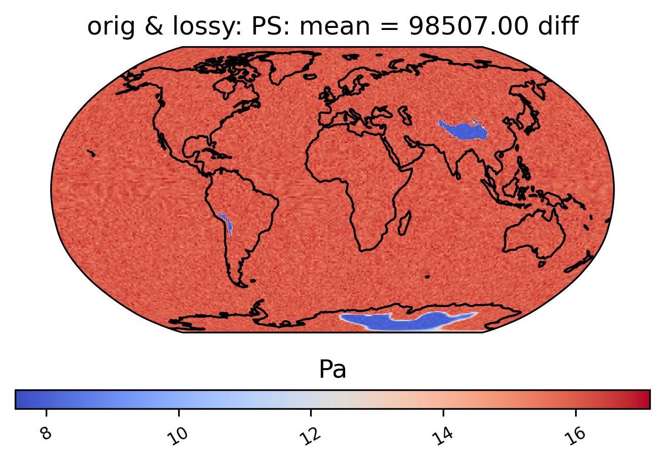
Now we instead show the difference plot for the above plots.
[12]:
# diff between mean PS values in col_PS orig and lossy datasets
ldcpy.plot(col_PS, "PS", sets=["orig", "lossy"], calc="mean", calc_type="diff")
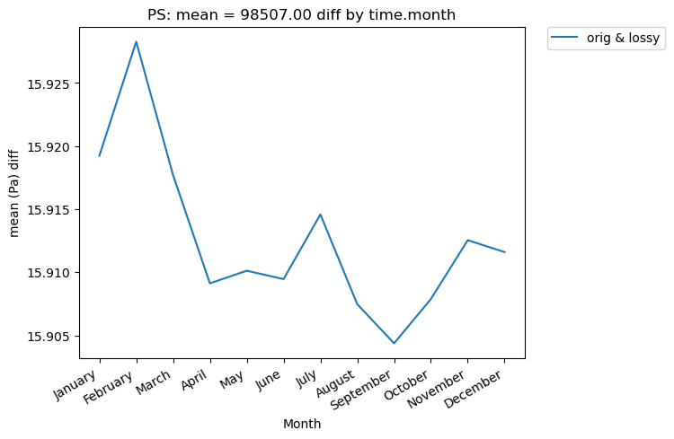
We can also look at mean differences over time. Here we are looking at the spatial averages and then grouping by day of the year. If doing a timeseries plot for this much data, using “group_by” is often a good idea.
[13]:
# Time-series plot of mean PS differences between col_PS orig and col_PS lossy datasets grouped by month of year
ldcpy.plot(
    col_PS,
    "PS",
    sets=["orig", "lossy"],
    calc="mean",
    plot_type="time_series",
    group_by="time.month",
    calc_type="diff",
)
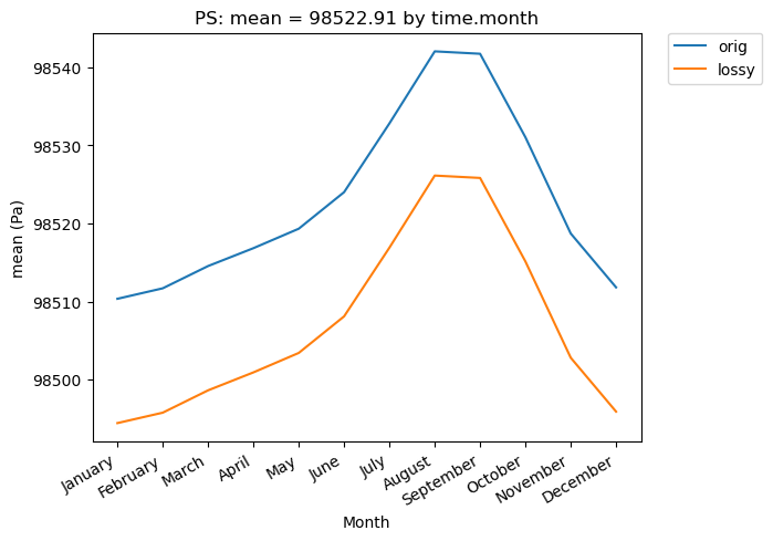
[14]:
# Time-series plot of PS mean (grouped by month) in the original and lossy datasets
ldcpy.plot(
    col_PS,
    "PS",
    sets=["orig", "lossy"],
    calc="mean",
    plot_type="time_series",
    group_by="time.month",
)
[15]:
del col_PS
Surface Temperature
Now let’s open the daily surface temperature (TS) data for 1920-2005 into a collection. These are larger files than the monthly PS data.
[16]:
# load the first 86 years of daily surface temperature (TS) data
col_TS = ldcpy.open_datasets(
    "cam-fv",
    ["TS"],
    [
        "/glade/p/cisl/asap/ldcpy_sample_data/lens/orig/TS.daily.19200101-20051231.nc",
        "/glade/p/cisl/asap/ldcpy_sample_data/lens/lossy/c.TS.daily.19200101-20051231.nc",
    ],
    ["orig", "lossy"],
    chunks={"time": 500},
)
col_TS
dataset size in GB 13.89
[16]:
<xarray.Dataset>
Dimensions:     (collection: 2, lat: 192, lon: 288, time: 31390)
Coordinates:
  * lat         (lat) float64 -90.0 -89.06 -88.12 -87.17 ... 88.12 89.06 90.0
  * lon         (lon) float64 0.0 1.25 2.5 3.75 5.0 ... 355.0 356.2 357.5 358.8
  * time        (time) object 1920-01-01 00:00:00 ... 2005-12-31 00:00:00
    cell_area   (lat, collection, lon) float64 dask.array<chunksize=(192, 1, 288), meta=np.ndarray>
  * collection  (collection) <U5 'orig' 'lossy'
Data variables:
    TS          (collection, time, lat, lon) float32 dask.array<chunksize=(1, 500, 192, 288), meta=np.ndarray>
Attributes:
    Conventions:      CF-1.0
    source:           CAM
    case:             b.e11.B20TRC5CNBDRD.f09_g16.031
    title:            UNSET
    logname:          mickelso
    host:             ys0219
    Version:          $Name$
    revision_Id:      $Id$
    initial_file:     b.e11.B20TRC5CNBDRD.f09_g16.001.cam.i.1920-01-01-00000.nc
    topography_file:  /glade/p/cesmdata/cseg/inputdata/atm/cam/topo/USGS-gtop...
    history:          Tue Nov  3 13:56:03 2020: ncks -L 5 TS.daily.19200101-2...
    NCO:              netCDF Operators version 4.7.9 (Homepage = http://nco.s...
    cell_measures:    area: cell_area
data_type: cam-fv- collection: 2
- lat: 192
- lon: 288
- time: 31390
- lat(lat)float64-90.0 -89.06 -88.12 ... 89.06 90.0
- long_name :
- latitude
- units :
- degrees_north
array([-90. , -89.057592, -88.115183, -87.172775, -86.230366, -85.287958, -84.34555 , -83.403141, -82.460733, -81.518325, -80.575916, -79.633508, -78.691099, -77.748691, -76.806283, -75.863874, -74.921466, -73.979058, -73.036649, -72.094241, -71.151832, -70.209424, -69.267016, -68.324607, -67.382199, -66.439791, -65.497382, -64.554974, -63.612565, -62.670157, -61.727749, -60.78534 , -59.842932, -58.900524, -57.958115, -57.015707, -56.073298, -55.13089 , -54.188482, -53.246073, -52.303665, -51.361257, -50.418848, -49.47644 , -48.534031, -47.591623, -46.649215, -45.706806, -44.764398, -43.82199 , -42.879581, -41.937173, -40.994764, -40.052356, -39.109948, -38.167539, -37.225131, -36.282723, -35.340314, -34.397906, -33.455497, -32.513089, -31.570681, -30.628272, -29.685864, -28.743455, -27.801047, -26.858639, -25.91623 , -24.973822, -24.031414, -23.089005, -22.146597, -21.204188, -20.26178 , -19.319372, -18.376963, -17.434555, -16.492147, -15.549738, -14.60733 , -13.664921, -12.722513, -11.780105, -10.837696, -9.895288, -8.95288 , -8.010471, -7.068063, -6.125654, -5.183246, -4.240838, -3.298429, -2.356021, -1.413613, -0.471204, 0.471204, 1.413613, 2.356021, 3.298429, 4.240838, 5.183246, 6.125654, 7.068063, 8.010471, 8.95288 , 9.895288, 10.837696, 11.780105, 12.722513, 13.664921, 14.60733 , 15.549738, 16.492147, 17.434555, 18.376963, 19.319372, 20.26178 , 21.204188, 22.146597, 23.089005, 24.031414, 24.973822, 25.91623 , 26.858639, 27.801047, 28.743455, 29.685864, 30.628272, 31.570681, 32.513089, 33.455497, 34.397906, 35.340314, 36.282723, 37.225131, 38.167539, 39.109948, 40.052356, 40.994764, 41.937173, 42.879581, 43.82199 , 44.764398, 45.706806, 46.649215, 47.591623, 48.534031, 49.47644 , 50.418848, 51.361257, 52.303665, 53.246073, 54.188482, 55.13089 , 56.073298, 57.015707, 57.958115, 58.900524, 59.842932, 60.78534 , 61.727749, 62.670157, 63.612565, 64.554974, 65.497382, 66.439791, 67.382199, 68.324607, 69.267016, 70.209424, 71.151832, 72.094241, 73.036649, 73.979058, 74.921466, 75.863874, 76.806283, 77.748691, 78.691099, 79.633508, 80.575916, 81.518325, 82.460733, 83.403141, 84.34555 , 85.287958, 86.230366, 87.172775, 88.115183, 89.057592, 90. ]) - lon(lon)float640.0 1.25 2.5 ... 356.2 357.5 358.8
- long_name :
- longitude
- units :
- degrees_east
array([ 0. , 1.25, 2.5 , ..., 356.25, 357.5 , 358.75])
- time(time)object1920-01-01 00:00:00 ... 2005-12-...
- long_name :
- time
- bounds :
- time_bnds
array([cftime.DatetimeNoLeap(1920, 1, 1, 0, 0, 0, 0), cftime.DatetimeNoLeap(1920, 1, 2, 0, 0, 0, 0), cftime.DatetimeNoLeap(1920, 1, 3, 0, 0, 0, 0), ..., cftime.DatetimeNoLeap(2005, 12, 29, 0, 0, 0, 0), cftime.DatetimeNoLeap(2005, 12, 30, 0, 0, 0, 0), cftime.DatetimeNoLeap(2005, 12, 31, 0, 0, 0, 0)], dtype=object) - cell_area(lat, collection, lon)float64dask.array<chunksize=(192, 1, 288), meta=np.ndarray>
- long_name :
- gauss weights
Array Chunk Bytes 884.74 kB 442.37 kB Shape (192, 2, 288) (192, 1, 288) Count 12 Tasks 2 Chunks Type float64 numpy.ndarray - collection(collection)<U5'orig' 'lossy'
array(['orig', 'lossy'], dtype='<U5')
- TS(collection, time, lat, lon)float32dask.array<chunksize=(1, 500, 192, 288), meta=np.ndarray>
- units :
- K
- long_name :
- Surface temperature (radiative)
- cell_methods :
- time: mean
Array Chunk Bytes 13.89 GB 110.59 MB Shape (2, 31390, 192, 288) (1, 500, 192, 288) Count 380 Tasks 126 Chunks Type float32 numpy.ndarray
- Conventions :
- CF-1.0
- source :
- CAM
- case :
- b.e11.B20TRC5CNBDRD.f09_g16.031
- title :
- UNSET
- logname :
- mickelso
- host :
- ys0219
- Version :
- $Name$
- revision_Id :
- $Id$
- initial_file :
- b.e11.B20TRC5CNBDRD.f09_g16.001.cam.i.1920-01-01-00000.nc
- topography_file :
- /glade/p/cesmdata/cseg/inputdata/atm/cam/topo/USGS-gtopo30_0.9x1.25_remap_c051027.nc
- history :
- Tue Nov 3 13:56:03 2020: ncks -L 5 TS.daily.19200101-20051231.nc T.nc Wed Aug 26 12:48:18 2020: ncks -d time,0,31389,1 TS.daily.19200101-20051231.nc new.TS.daily.19200101-20051231.nc
- NCO :
- netCDF Operators version 4.7.9 (Homepage = http://nco.sf.net, Code = http://github.com/nco/nco)
- cell_measures :
- area: cell_area
- data_type :
- cam-fv
Look at the first time slice (time = 0) statistics:
[17]:
ldcpy.compare_stats(col_TS.isel(time=0), "TS", ["orig", "lossy"])
| orig | lossy | |
|---|---|---|
| mean | 274.71 | 274.66 |
| variance | 533.98 | 533.43 |
| standard deviation | 23.108 | 23.096 |
| min value | 315.58 | 315.5 |
| max value | 216.73 | 216.69 |
| probability positive | 1 | 1 |
| number of zeros | 0 | 0 |
| lossy | |
|---|---|
| max abs diff | 0.12497 |
| min abs diff | 0 |
| mean abs diff | 0.054906 |
| mean squared diff | 0.0030146 |
| root mean squared diff | 0.06527 |
| normalized root mean squared diff | 0.0006603 |
| normalized max pointwise error | 0.0012642 |
| pearson correlation coefficient | 1 |
| ks p-value | 0.36817 |
| spatial relative error(% > 0.0001) | 73.293 |
| max spatial relative error | 0.00048733 |
| Data SSIM | 0.97883 |
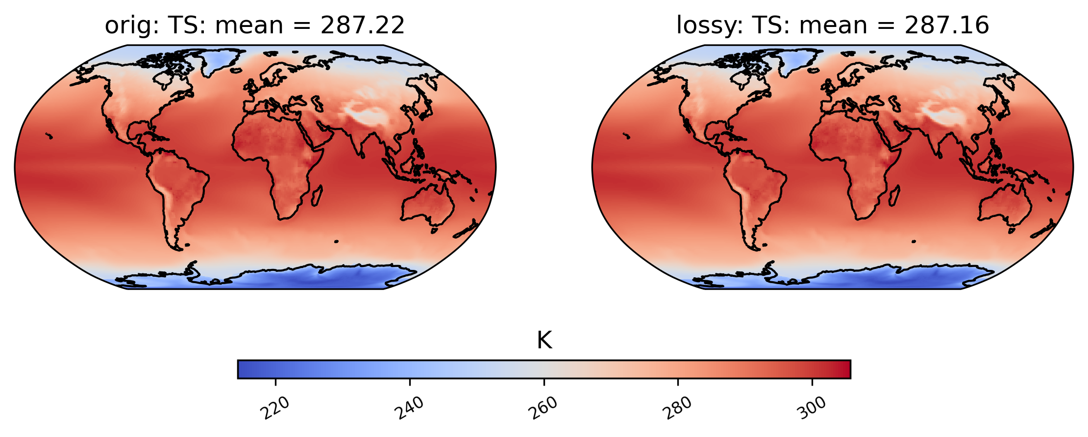
Now we compare mean TS over time in a plot:
[18]:
# comparison between mean TS values in col_TS orig and lossy datasets
ldcpy.plot(col_TS, "TS", sets=["orig", "lossy"], calc="mean")
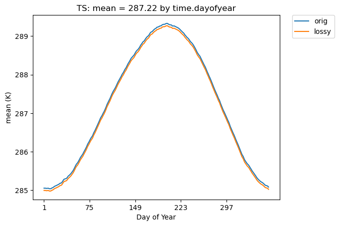
Below we do a time series plot and group by day of the year. (Note that the group_by functionality is not fast.)
[19]:
# Time-series plot of TS means (grouped by days) in the original and lossy datasets
ldcpy.plot(
    col_TS,
    "TS",
    sets=["orig", "lossy"],
    calc="mean",
    plot_type="time_series",
    group_by="time.dayofyear",
)
Let’s delete the PS and TS data to free up memory.
[20]:
del col_TS
Precipitation Rate
Now let’s open the daily precipitation rate (PRECT) data for 2006-2080 into a collection.
[21]:
# load the last 75 years of PRECT data
col_PRECT = ldcpy.open_datasets(
    "cam-fv",
    ["PRECT"],
    [
        "/glade/p/cisl/asap/ldcpy_sample_data/lens/orig/PRECT.daily.20060101-20801231.nc",
        "/glade/p/cisl/asap/ldcpy_sample_data/lens/lossy/c.PRECT.daily.20060101-20801231.nc",
    ],
    ["orig", "lossy"],
    chunks={"time": 500},
)
col_PRECT
dataset size in GB 12.11
[21]:
<xarray.Dataset>
Dimensions:     (collection: 2, lat: 192, lon: 288, time: 27375)
Coordinates:
  * lat         (lat) float64 -90.0 -89.06 -88.12 -87.17 ... 88.12 89.06 90.0
  * lon         (lon) float64 0.0 1.25 2.5 3.75 5.0 ... 355.0 356.2 357.5 358.8
  * time        (time) object 2006-01-01 00:00:00 ... 2080-12-31 00:00:00
    cell_area   (lat, collection, lon) float64 dask.array<chunksize=(192, 1, 288), meta=np.ndarray>
  * collection  (collection) <U5 'orig' 'lossy'
Data variables:
    PRECT       (collection, time, lat, lon) float32 dask.array<chunksize=(1, 500, 192, 288), meta=np.ndarray>
Attributes:
    Conventions:      CF-1.0
    source:           CAM
    case:             b.e11.BRCP85C5CNBDRD.f09_g16.031
    title:            UNSET
    logname:          mickelso
    host:             ys1023
    Version:          $Name$
    revision_Id:      $Id$
    initial_file:     b.e11.B20TRC5CNBDRD.f09_g16.031.cam.i.2006-01-01-00000.nc
    topography_file:  /glade/p/cesmdata/cseg/inputdata/atm/cam/topo/USGS-gtop...
    history:          Tue Nov  3 14:13:51 2020: ncks -L 5 PRECT.daily.2006010...
    NCO:              netCDF Operators version 4.7.9 (Homepage = http://nco.s...
    cell_measures:    area: cell_area
data_type: cam-fv- collection: 2
- lat: 192
- lon: 288
- time: 27375
- lat(lat)float64-90.0 -89.06 -88.12 ... 89.06 90.0
- long_name :
- latitude
- units :
- degrees_north
array([-90. , -89.057592, -88.115183, -87.172775, -86.230366, -85.287958, -84.34555 , -83.403141, -82.460733, -81.518325, -80.575916, -79.633508, -78.691099, -77.748691, -76.806283, -75.863874, -74.921466, -73.979058, -73.036649, -72.094241, -71.151832, -70.209424, -69.267016, -68.324607, -67.382199, -66.439791, -65.497382, -64.554974, -63.612565, -62.670157, -61.727749, -60.78534 , -59.842932, -58.900524, -57.958115, -57.015707, -56.073298, -55.13089 , -54.188482, -53.246073, -52.303665, -51.361257, -50.418848, -49.47644 , -48.534031, -47.591623, -46.649215, -45.706806, -44.764398, -43.82199 , -42.879581, -41.937173, -40.994764, -40.052356, -39.109948, -38.167539, -37.225131, -36.282723, -35.340314, -34.397906, -33.455497, -32.513089, -31.570681, -30.628272, -29.685864, -28.743455, -27.801047, -26.858639, -25.91623 , -24.973822, -24.031414, -23.089005, -22.146597, -21.204188, -20.26178 , -19.319372, -18.376963, -17.434555, -16.492147, -15.549738, -14.60733 , -13.664921, -12.722513, -11.780105, -10.837696, -9.895288, -8.95288 , -8.010471, -7.068063, -6.125654, -5.183246, -4.240838, -3.298429, -2.356021, -1.413613, -0.471204, 0.471204, 1.413613, 2.356021, 3.298429, 4.240838, 5.183246, 6.125654, 7.068063, 8.010471, 8.95288 , 9.895288, 10.837696, 11.780105, 12.722513, 13.664921, 14.60733 , 15.549738, 16.492147, 17.434555, 18.376963, 19.319372, 20.26178 , 21.204188, 22.146597, 23.089005, 24.031414, 24.973822, 25.91623 , 26.858639, 27.801047, 28.743455, 29.685864, 30.628272, 31.570681, 32.513089, 33.455497, 34.397906, 35.340314, 36.282723, 37.225131, 38.167539, 39.109948, 40.052356, 40.994764, 41.937173, 42.879581, 43.82199 , 44.764398, 45.706806, 46.649215, 47.591623, 48.534031, 49.47644 , 50.418848, 51.361257, 52.303665, 53.246073, 54.188482, 55.13089 , 56.073298, 57.015707, 57.958115, 58.900524, 59.842932, 60.78534 , 61.727749, 62.670157, 63.612565, 64.554974, 65.497382, 66.439791, 67.382199, 68.324607, 69.267016, 70.209424, 71.151832, 72.094241, 73.036649, 73.979058, 74.921466, 75.863874, 76.806283, 77.748691, 78.691099, 79.633508, 80.575916, 81.518325, 82.460733, 83.403141, 84.34555 , 85.287958, 86.230366, 87.172775, 88.115183, 89.057592, 90. ]) - lon(lon)float640.0 1.25 2.5 ... 356.2 357.5 358.8
- long_name :
- longitude
- units :
- degrees_east
array([ 0. , 1.25, 2.5 , ..., 356.25, 357.5 , 358.75])
- time(time)object2006-01-01 00:00:00 ... 2080-12-...
- long_name :
- time
- bounds :
- time_bnds
array([cftime.DatetimeNoLeap(2006, 1, 1, 0, 0, 0, 0), cftime.DatetimeNoLeap(2006, 1, 2, 0, 0, 0, 0), cftime.DatetimeNoLeap(2006, 1, 3, 0, 0, 0, 0), ..., cftime.DatetimeNoLeap(2080, 12, 29, 0, 0, 0, 0), cftime.DatetimeNoLeap(2080, 12, 30, 0, 0, 0, 0), cftime.DatetimeNoLeap(2080, 12, 31, 0, 0, 0, 0)], dtype=object) - cell_area(lat, collection, lon)float64dask.array<chunksize=(192, 1, 288), meta=np.ndarray>
- long_name :
- gauss weights
Array Chunk Bytes 884.74 kB 442.37 kB Shape (192, 2, 288) (192, 1, 288) Count 12 Tasks 2 Chunks Type float64 numpy.ndarray - collection(collection)<U5'orig' 'lossy'
array(['orig', 'lossy'], dtype='<U5')
- PRECT(collection, time, lat, lon)float32dask.array<chunksize=(1, 500, 192, 288), meta=np.ndarray>
- units :
- m/s
- long_name :
- Total (convective and large-scale) precipitation rate (liq + ice)
- cell_methods :
- time: mean
Array Chunk Bytes 12.11 GB 110.59 MB Shape (2, 27375, 192, 288) (1, 500, 192, 288) Count 332 Tasks 110 Chunks Type float32 numpy.ndarray
- Conventions :
- CF-1.0
- source :
- CAM
- case :
- b.e11.BRCP85C5CNBDRD.f09_g16.031
- title :
- UNSET
- logname :
- mickelso
- host :
- ys1023
- Version :
- $Name$
- revision_Id :
- $Id$
- initial_file :
- b.e11.B20TRC5CNBDRD.f09_g16.031.cam.i.2006-01-01-00000.nc
- topography_file :
- /glade/p/cesmdata/cseg/inputdata/atm/cam/topo/USGS-gtopo30_0.9x1.25_remap_c051027.nc
- history :
- Tue Nov 3 14:13:51 2020: ncks -L 5 PRECT.daily.20060101-20801231.nc P2006.nc Wed Aug 26 13:13:19 2020: ncks -d time,0,27374,1 PRECT.daily.20060101-20801231.nc new.PRECT.daily.20060101-20801231.nc
- NCO :
- netCDF Operators version 4.7.9 (Homepage = http://nco.sf.net, Code = http://github.com/nco/nco)
- cell_measures :
- area: cell_area
- data_type :
- cam-fv
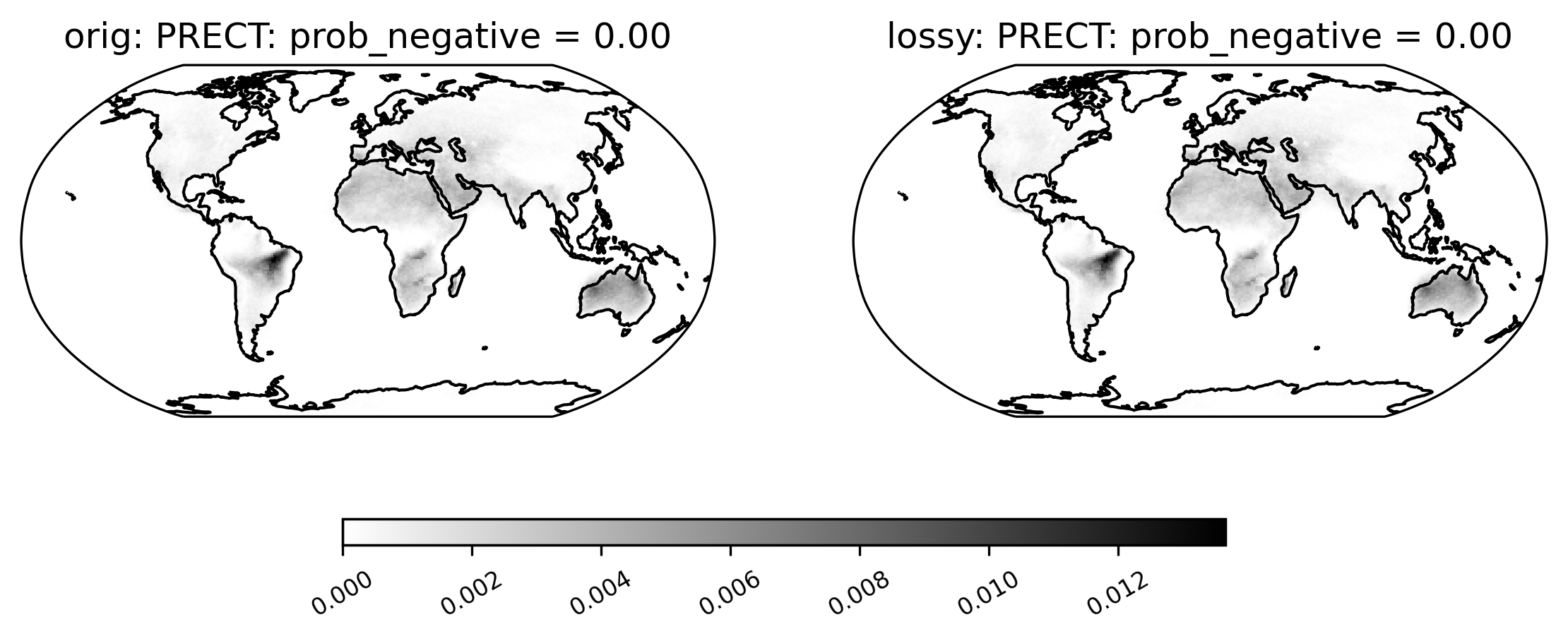
[22]:
# compare probability of negative rainfall (and get ssim)
ldcpy.plot(
    col_PRECT,
    "PRECT",
    sets=["orig", "lossy"],
    calc="prob_negative",
    color="binary",
    calc_ssim=True,
)
SSIM 1 & 2 = 1.00000
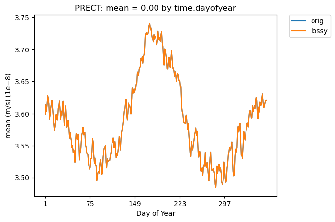
Mean PRECT over time…
[23]:
# Time-series plot of PRECT mean in 'orig' dataset
ldcpy.plot(
    col_PRECT,
    "PRECT",
    sets=["orig", "lossy"],
    calc="mean",
    plot_type="time_series",
    group_by="time.dayofyear",
)
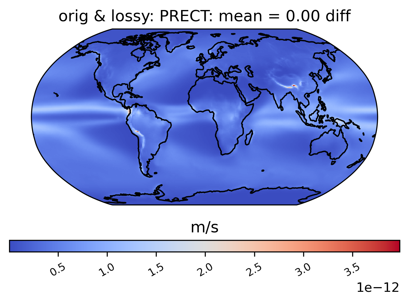
Now look at mean over time spatial plot:
[24]:
# diff between mean PRECT values across the entire timeseries
ldcpy.plot(
    col_PRECT,
    "PRECT",
    sets=["orig", "lossy"],
    calc="mean",
    calc_type="diff",
)
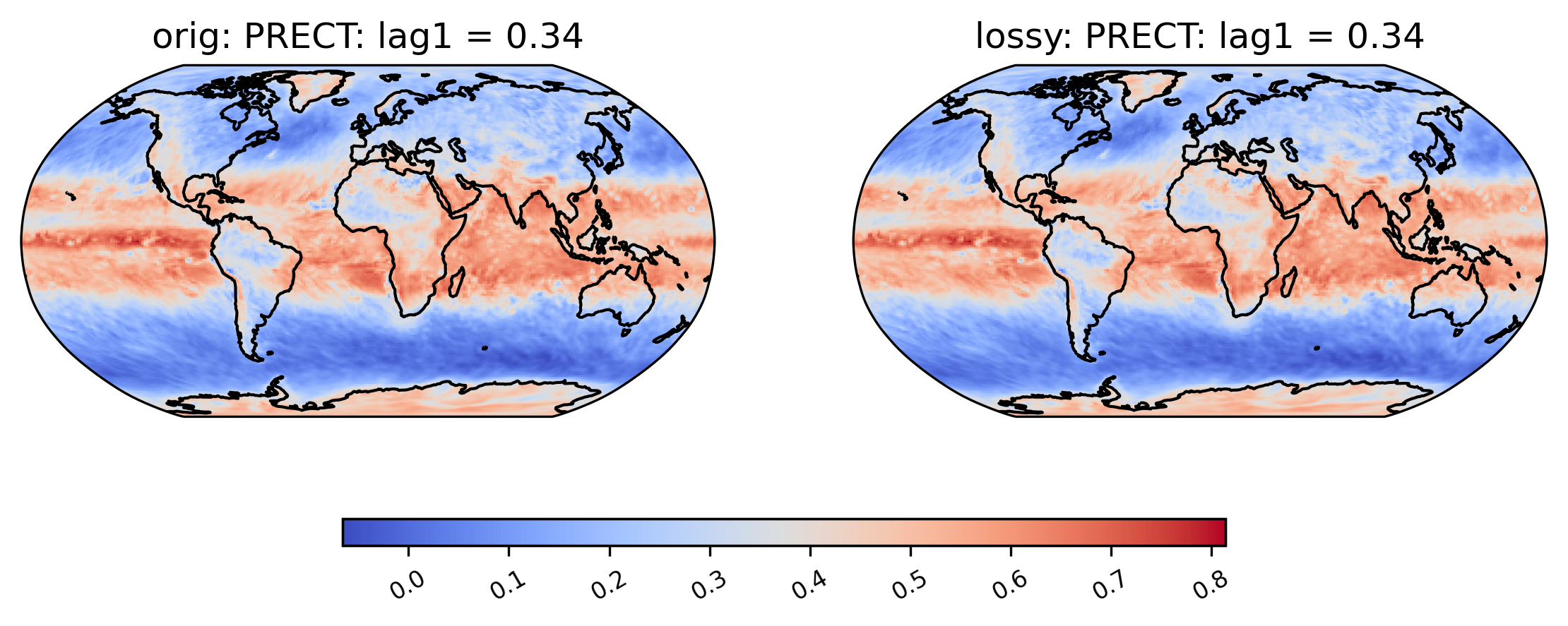
Calculating the correlation of the lag-1 values … for the first 10 years (This operation can be time-consuming).
[25]:
# plot of lag-1 correlation of PRECT values
ldcpy.plot(col_PRECT, "PRECT", sets=["orig", "lossy"], calc="lag1", start=0, end=3650)
CAGEO Plots
Comparing the sz and zfp compressors with a number of metrics (specified with “calc” and “calc_type” in the plot routine).
[26]:
col_TS = ldcpy.open_datasets(
    "cam-fv",
    ["TS"],
    [
        "/glade/p/cisl/asap/ldcpy_sample_data/cageo/orig/b.e11.B20TRC5CNBDRD.f09_g16.030.cam.h1.TS.19200101-20051231.nc",
        "/glade/p/cisl/asap/ldcpy_sample_data/cageo/lossy/sz1.0.TS.nc",
        "/glade/p/cisl/asap/ldcpy_sample_data/cageo/lossy/zfp1.0.TS.nc",
    ],
    ["orig", "sz1.0", "zfp1.0"],
    chunks={"time": 500},
)
col_PRECT = ldcpy.open_datasets(
    "cam-fv",
    ["PRECT"],
    [
        "/glade/p/cisl/asap/ldcpy_sample_data/cageo/orig/b.e11.B20TRC5CNBDRD.f09_g16.030.cam.h1.PRECT.19200101-20051231.nc",
        "/glade/p/cisl/asap/ldcpy_sample_data/cageo/lossy/sz1e-8.PRECT.nc",
        "/glade/p/cisl/asap/ldcpy_sample_data/cageo/lossy/zfp1e-8.PRECT.nc",
    ],
    ["orig", "sz1e-8", "zfp1e-8"],
    chunks={"time": 500},
)
dataset size in GB 20.83

dataset size in GB 20.83
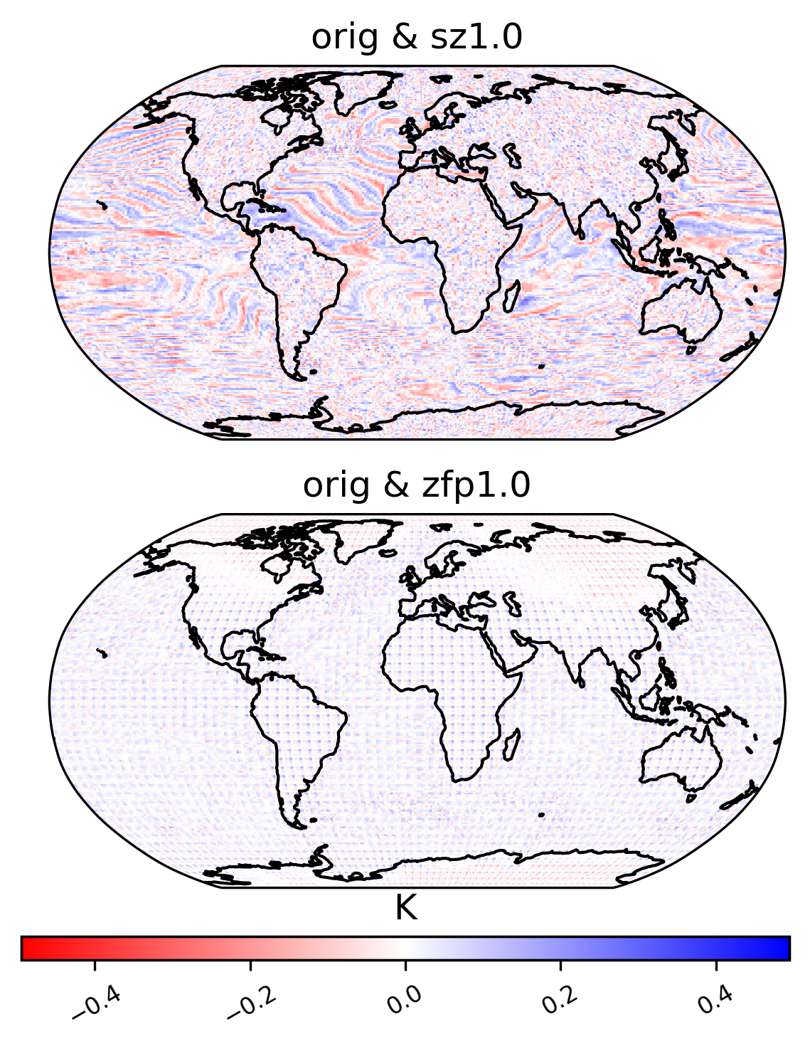
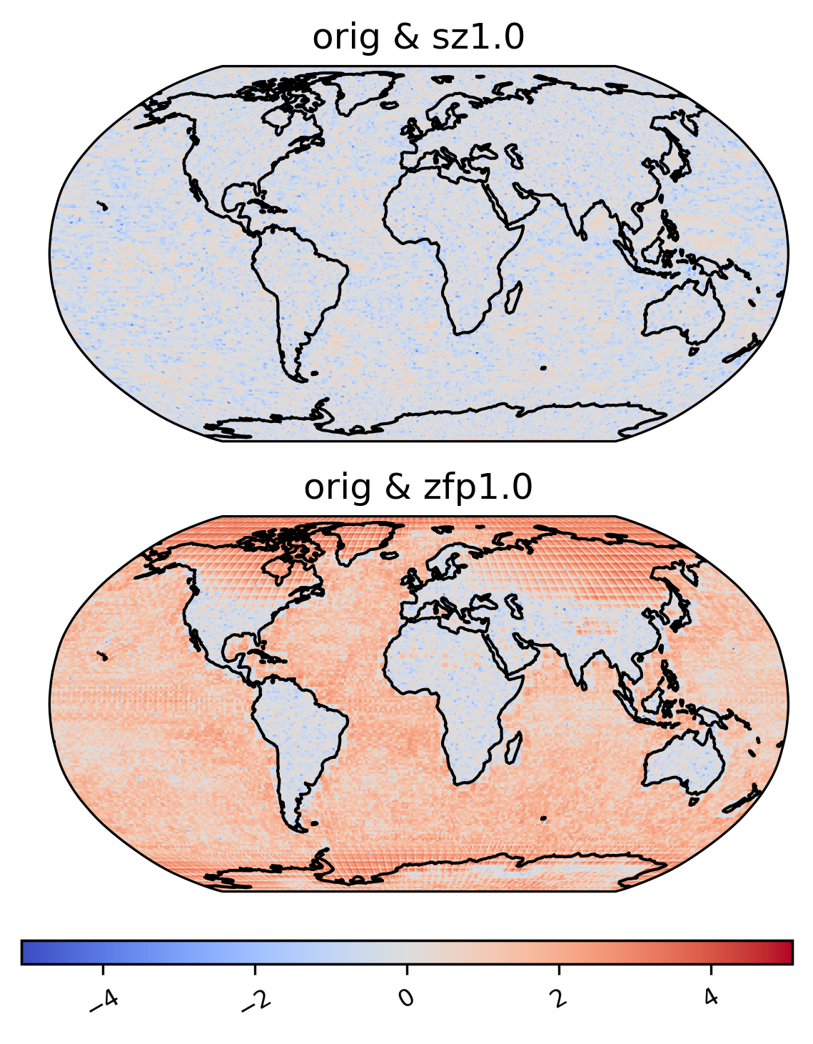
difference in mean
[27]:
ldcpy.plot(
    col_TS,
    "TS",
    sets=["orig", "sz1.0", "zfp1.0"],
    calc="mean",
    calc_type="diff",
    color="bwr_r",
    start=0,
    end=50,
    tex_format=False,
    vert_plot=True,
    short_title=True,
    axes_symmetric=True,
)
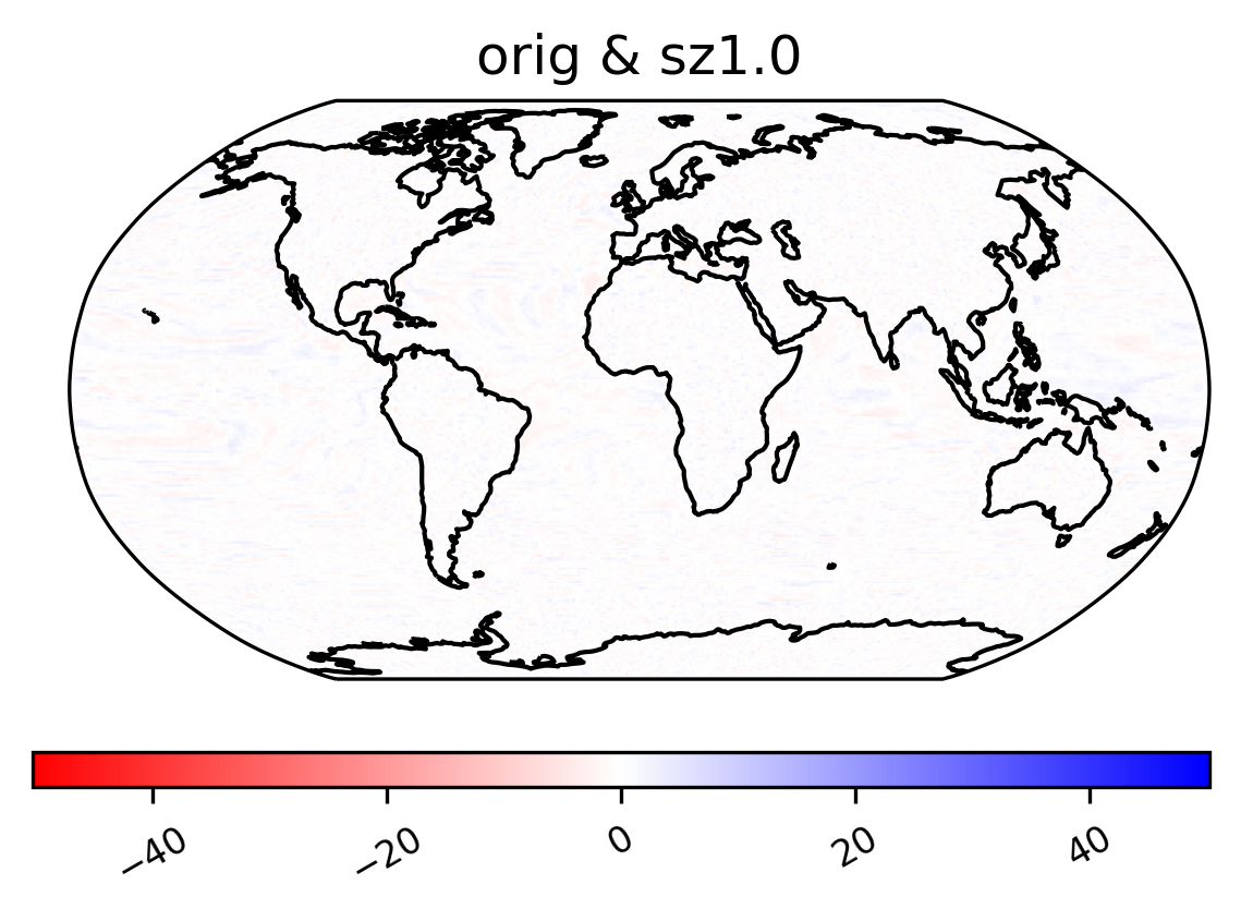
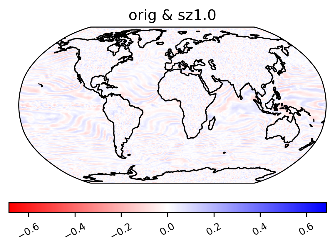
Zscore
[28]:
ldcpy.plot(
    col_TS,
    "TS",
    sets=["orig", "sz1.0"],
    calc="zscore",
    calc_type="calc_of_diff",
    color="bwr_r",
    start=0,
    end=1000,
    tex_format=False,
    vert_plot=True,
    short_title=True,
    axes_symmetric=True,
)
Pooled variance ratio
[29]:
ldcpy.plot(
    col_TS,
    "TS",
    sets=["orig", "sz1.0"],
    calc="pooled_var_ratio",
    color="bwr_r",
    calc_type="calc_of_diff",
    transform="log",
    start=0,
    end=100,
    tex_format=False,
    vert_plot=True,
    short_title=True,
    axes_symmetric=True,
)
annual harmonic relative ratio
[30]:
col_TS["TS"] = col_TS.TS.chunk({"time": -1, "lat": 10, "lon": 10})
ldcpy.plot(
    col_TS,
    "TS",
    sets=["orig", "sz1.0", "zfp1.0"],
    calc="ann_harmonic_ratio",
    transform="log",
    calc_type="calc_of_diff",
    tex_format=False,
    axes_symmetric=True,
    vert_plot=True,
    short_title=True,
)
col_TS["TS"] = col_TS.TS.chunk({"time": 500, "lat": 192, "lon": 288})
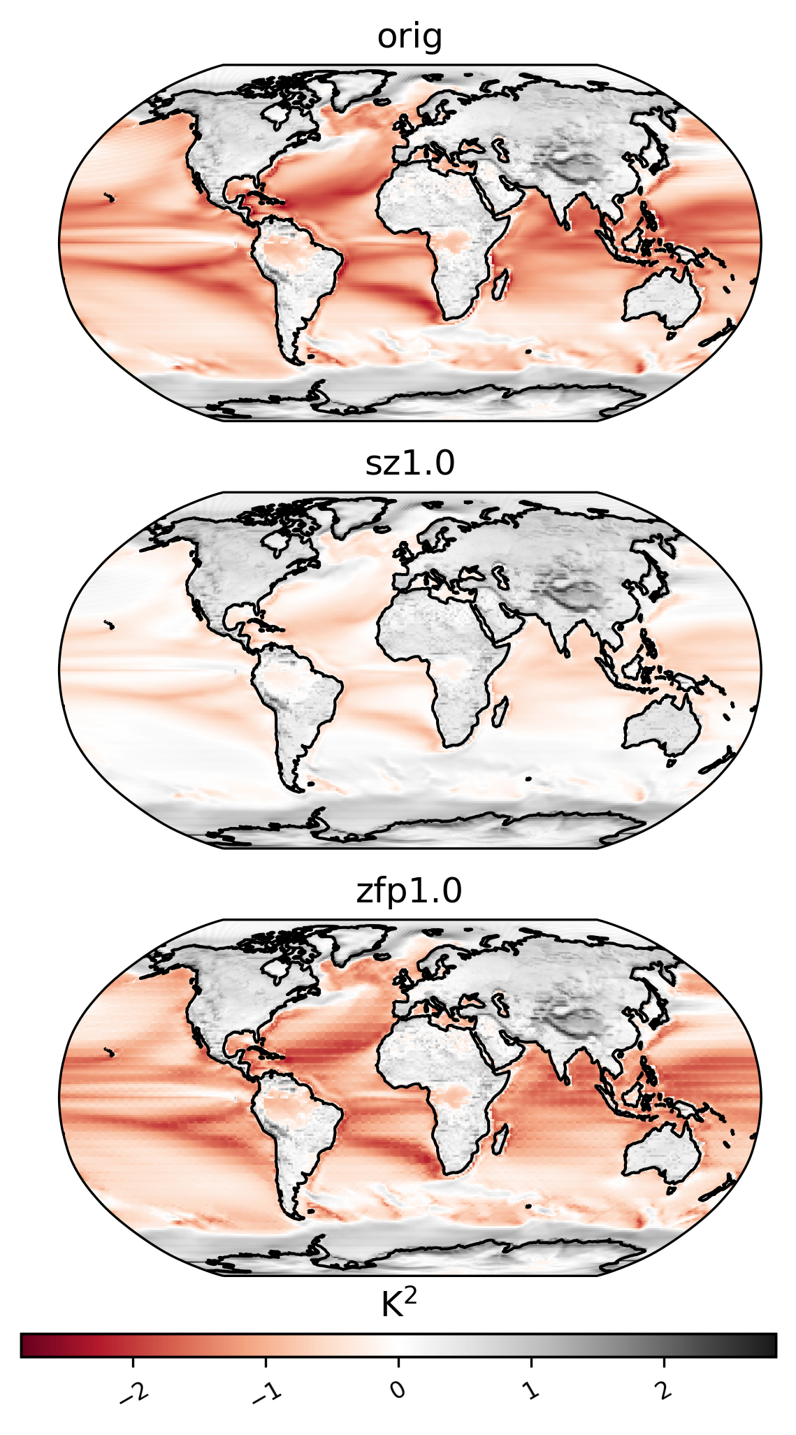
NS contrast variance
[31]:
ldcpy.plot(
    col_TS,
    "TS",
    sets=["orig", "sz1.0", "zfp1.0"],
    calc="ns_con_var",
    color="RdGy",
    calc_type="raw",
    transform="log",
    axes_symmetric=True,
    tex_format=False,
    vert_plot=True,
    short_title=True,
)
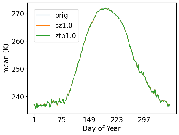
mean by day of year
[32]:
ldcpy.plot(
    col_TS,
    "TS",
    sets=["orig", "sz1.0", "zfp1.0"],
    calc="mean",
    plot_type="time_series",
    group_by="time.dayofyear",
    legend_loc="upper left",
    lat=90,
    lon=0,
    vert_plot=True,
    tex_format=False,
    short_title=True,
)
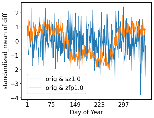
standardized mean errors by day of year
[33]:
ldcpy.plot(
    col_TS,
    "TS",
    sets=["orig", "sz1.0", "zfp1.0"],
    calc="standardized_mean",
    legend_loc="lower left",
    calc_type="calc_of_diff",
    plot_type="time_series",
    group_by="time.dayofyear",
    tex_format=False,
    lat=90,
    lon=0,
    vert_plot=True,
    short_title=True,
)
[34]:
del col_TS
Do any other comparisons you wish … and then clean up!
[ ]:
client.close()