Using data from AWS
A significant amount of Earth System Model (ESM) data is publicly available online, including data from the CESM Large Ensemble, CMIP5, and CMIP6 datasets. For accessing a single file, we can specify the file (typically netcdf or zarr format) and its location and then use fsspec (the “Filesystem Spec+ python package) and xarray to create a array.dataset. For several files, the intake_esm python module (https://github.com/intake/intake-esm) is particularly nice for obtaining the data and put it into an xarray.dataset.
This notebook assumes familiarity with the Tutorial Notebook. It additionally shows how to gather data from an ESM collection, put it into a dataset, and then create simple plots using the data with ldcpy.
Example Data
The example data we use is from the CESM Large Ensemble, member 31. This ensemble data has been lossily compressed and reconstructed as part of a blind evaluation study of lossy data compression in LENS (e.g., http://www.cesm.ucar.edu/projects/community-projects/LENS/projects/lossy-data-compression.html or https://gmd.copernicus.org/articles/9/4381/2016/).
Most of the data from the CESM Large Ensemble Project has been made available on Amazon Web Services (Amazon S3), see http://ncar-aws-www.s3-website-us-west-2.amazonaws.com/CESM_LENS_on_AWS.htm .
For comparison purposes, the original (non-compressed) data for Ensemble 31 has recently been made available on Amazon Web Services (Amazon S3) in the “ncar-cesm-lens-baker-lossy-compression-test” bucket.
[1]:
# Add ldcpy root to system path
# Using kernel 2024b
import sys

sys.path.insert(0, '../../../')

# Import ldcpy package
# Autoreloads package everytime the package is called, so changes to code will be reflected in the notebook if the above sys.path.insert(...) line is uncommented.
%load_ext autoreload
%autoreload 2
import fsspec
import intake
import xarray as xr

import ldcpy

# display the plots in this notebook
%matplotlib inline

# silence warnings
import warnings

warnings.filterwarnings("ignore")
First, specify the filesystem and location of the data. Here we are accessing the original data from CESM-LENS ensemble 31, which is available on Amazon S3 in the store named “ncar-cesm-lens-baker-lossy-compression-test” bucket.
First we listing all available files (which are timeseries files containing a single variable) for that dataset. Note that unlike in the TutorialNotebook (which used NetCDF files), these files are all zarr format. Both monthly and daily data is available.
[2]:
fs = fsspec.filesystem("s3", anon=True)
stores = fs.ls("ncar-cesm-lens-baker-lossy-compression-test/lens-ens31/")[1:]
stores[:]
[2]:
['ncar-cesm-lens-baker-lossy-compression-test/lens-ens31/cesmle-atm-ens31-20C-daily-FLNS.zarr',
 'ncar-cesm-lens-baker-lossy-compression-test/lens-ens31/cesmle-atm-ens31-20C-daily-FLNSC.zarr',
 'ncar-cesm-lens-baker-lossy-compression-test/lens-ens31/cesmle-atm-ens31-20C-daily-FLUT.zarr',
 'ncar-cesm-lens-baker-lossy-compression-test/lens-ens31/cesmle-atm-ens31-20C-daily-FSNS.zarr',
 'ncar-cesm-lens-baker-lossy-compression-test/lens-ens31/cesmle-atm-ens31-20C-daily-FSNSC.zarr',
 'ncar-cesm-lens-baker-lossy-compression-test/lens-ens31/cesmle-atm-ens31-20C-daily-FSNTOA.zarr',
 'ncar-cesm-lens-baker-lossy-compression-test/lens-ens31/cesmle-atm-ens31-20C-daily-ICEFRAC.zarr',
 'ncar-cesm-lens-baker-lossy-compression-test/lens-ens31/cesmle-atm-ens31-20C-daily-LHFLX.zarr',
 'ncar-cesm-lens-baker-lossy-compression-test/lens-ens31/cesmle-atm-ens31-20C-daily-PRECL.zarr',
 'ncar-cesm-lens-baker-lossy-compression-test/lens-ens31/cesmle-atm-ens31-20C-daily-PRECSC.zarr',
 'ncar-cesm-lens-baker-lossy-compression-test/lens-ens31/cesmle-atm-ens31-20C-daily-PRECSL.zarr',
 'ncar-cesm-lens-baker-lossy-compression-test/lens-ens31/cesmle-atm-ens31-20C-daily-PRECT.zarr',
 'ncar-cesm-lens-baker-lossy-compression-test/lens-ens31/cesmle-atm-ens31-20C-daily-PRECTMX.zarr',
 'ncar-cesm-lens-baker-lossy-compression-test/lens-ens31/cesmle-atm-ens31-20C-daily-PSL.zarr',
 'ncar-cesm-lens-baker-lossy-compression-test/lens-ens31/cesmle-atm-ens31-20C-daily-Q850.zarr',
 'ncar-cesm-lens-baker-lossy-compression-test/lens-ens31/cesmle-atm-ens31-20C-daily-SHFLX.zarr',
 'ncar-cesm-lens-baker-lossy-compression-test/lens-ens31/cesmle-atm-ens31-20C-daily-TMQ.zarr',
 'ncar-cesm-lens-baker-lossy-compression-test/lens-ens31/cesmle-atm-ens31-20C-daily-TREFHT.zarr',
 'ncar-cesm-lens-baker-lossy-compression-test/lens-ens31/cesmle-atm-ens31-20C-daily-TREFHTMN.zarr',
 'ncar-cesm-lens-baker-lossy-compression-test/lens-ens31/cesmle-atm-ens31-20C-daily-TREFHTMX.zarr',
 'ncar-cesm-lens-baker-lossy-compression-test/lens-ens31/cesmle-atm-ens31-20C-daily-TS.zarr',
 'ncar-cesm-lens-baker-lossy-compression-test/lens-ens31/cesmle-atm-ens31-20C-daily-UBOT.zarr',
 'ncar-cesm-lens-baker-lossy-compression-test/lens-ens31/cesmle-atm-ens31-20C-daily-WSPDSRFAV.zarr',
 'ncar-cesm-lens-baker-lossy-compression-test/lens-ens31/cesmle-atm-ens31-20C-daily-Z500.zarr',
 'ncar-cesm-lens-baker-lossy-compression-test/lens-ens31/cesmle-atm-ens31-20C-monthly-FLNS.zarr',
 'ncar-cesm-lens-baker-lossy-compression-test/lens-ens31/cesmle-atm-ens31-20C-monthly-FLNSC.zarr',
 'ncar-cesm-lens-baker-lossy-compression-test/lens-ens31/cesmle-atm-ens31-20C-monthly-FLUT.zarr',
 'ncar-cesm-lens-baker-lossy-compression-test/lens-ens31/cesmle-atm-ens31-20C-monthly-FSNS.zarr',
 'ncar-cesm-lens-baker-lossy-compression-test/lens-ens31/cesmle-atm-ens31-20C-monthly-FSNSC.zarr',
 'ncar-cesm-lens-baker-lossy-compression-test/lens-ens31/cesmle-atm-ens31-20C-monthly-FSNTOA.zarr',
 'ncar-cesm-lens-baker-lossy-compression-test/lens-ens31/cesmle-atm-ens31-20C-monthly-ICEFRAC.zarr',
 'ncar-cesm-lens-baker-lossy-compression-test/lens-ens31/cesmle-atm-ens31-20C-monthly-LHFLX.zarr',
 'ncar-cesm-lens-baker-lossy-compression-test/lens-ens31/cesmle-atm-ens31-20C-monthly-PRECC.zarr',
 'ncar-cesm-lens-baker-lossy-compression-test/lens-ens31/cesmle-atm-ens31-20C-monthly-PRECL.zarr',
 'ncar-cesm-lens-baker-lossy-compression-test/lens-ens31/cesmle-atm-ens31-20C-monthly-PRECSC.zarr',
 'ncar-cesm-lens-baker-lossy-compression-test/lens-ens31/cesmle-atm-ens31-20C-monthly-PRECSL.zarr',
 'ncar-cesm-lens-baker-lossy-compression-test/lens-ens31/cesmle-atm-ens31-20C-monthly-PSL.zarr',
 'ncar-cesm-lens-baker-lossy-compression-test/lens-ens31/cesmle-atm-ens31-20C-monthly-Q.zarr',
 'ncar-cesm-lens-baker-lossy-compression-test/lens-ens31/cesmle-atm-ens31-20C-monthly-SHFLX.zarr',
 'ncar-cesm-lens-baker-lossy-compression-test/lens-ens31/cesmle-atm-ens31-20C-monthly-T.zarr',
 'ncar-cesm-lens-baker-lossy-compression-test/lens-ens31/cesmle-atm-ens31-20C-monthly-TMQ.zarr',
 'ncar-cesm-lens-baker-lossy-compression-test/lens-ens31/cesmle-atm-ens31-20C-monthly-TREFHT.zarr',
 'ncar-cesm-lens-baker-lossy-compression-test/lens-ens31/cesmle-atm-ens31-20C-monthly-TREFHTMN.zarr',
 'ncar-cesm-lens-baker-lossy-compression-test/lens-ens31/cesmle-atm-ens31-20C-monthly-TREFHTMX.zarr',
 'ncar-cesm-lens-baker-lossy-compression-test/lens-ens31/cesmle-atm-ens31-20C-monthly-TS.zarr',
 'ncar-cesm-lens-baker-lossy-compression-test/lens-ens31/cesmle-atm-ens31-20C-monthly-U.zarr',
 'ncar-cesm-lens-baker-lossy-compression-test/lens-ens31/cesmle-atm-ens31-20C-monthly-V.zarr',
 'ncar-cesm-lens-baker-lossy-compression-test/lens-ens31/cesmle-atm-ens31-20C-monthly-Z3.zarr',
 'ncar-cesm-lens-baker-lossy-compression-test/lens-ens31/cesmle-atm-ens31-RCP85-daily-FLNS.zarr',
 'ncar-cesm-lens-baker-lossy-compression-test/lens-ens31/cesmle-atm-ens31-RCP85-daily-FLNSC.zarr',
 'ncar-cesm-lens-baker-lossy-compression-test/lens-ens31/cesmle-atm-ens31-RCP85-daily-FLUT.zarr',
 'ncar-cesm-lens-baker-lossy-compression-test/lens-ens31/cesmle-atm-ens31-RCP85-daily-FSNS.zarr',
 'ncar-cesm-lens-baker-lossy-compression-test/lens-ens31/cesmle-atm-ens31-RCP85-daily-FSNSC.zarr',
 'ncar-cesm-lens-baker-lossy-compression-test/lens-ens31/cesmle-atm-ens31-RCP85-daily-FSNTOA.zarr',
 'ncar-cesm-lens-baker-lossy-compression-test/lens-ens31/cesmle-atm-ens31-RCP85-daily-ICEFRAC.zarr',
 'ncar-cesm-lens-baker-lossy-compression-test/lens-ens31/cesmle-atm-ens31-RCP85-daily-LHFLX.zarr',
 'ncar-cesm-lens-baker-lossy-compression-test/lens-ens31/cesmle-atm-ens31-RCP85-daily-PRECL.zarr',
 'ncar-cesm-lens-baker-lossy-compression-test/lens-ens31/cesmle-atm-ens31-RCP85-daily-PRECSC.zarr',
 'ncar-cesm-lens-baker-lossy-compression-test/lens-ens31/cesmle-atm-ens31-RCP85-daily-PRECSL.zarr',
 'ncar-cesm-lens-baker-lossy-compression-test/lens-ens31/cesmle-atm-ens31-RCP85-daily-PRECT.zarr',
 'ncar-cesm-lens-baker-lossy-compression-test/lens-ens31/cesmle-atm-ens31-RCP85-daily-PRECTMX.zarr',
 'ncar-cesm-lens-baker-lossy-compression-test/lens-ens31/cesmle-atm-ens31-RCP85-daily-PSL.zarr',
 'ncar-cesm-lens-baker-lossy-compression-test/lens-ens31/cesmle-atm-ens31-RCP85-daily-Q850.zarr',
 'ncar-cesm-lens-baker-lossy-compression-test/lens-ens31/cesmle-atm-ens31-RCP85-daily-SHFLX.zarr',
 'ncar-cesm-lens-baker-lossy-compression-test/lens-ens31/cesmle-atm-ens31-RCP85-daily-TMQ.zarr',
 'ncar-cesm-lens-baker-lossy-compression-test/lens-ens31/cesmle-atm-ens31-RCP85-daily-TREFHT.zarr',
 'ncar-cesm-lens-baker-lossy-compression-test/lens-ens31/cesmle-atm-ens31-RCP85-daily-TREFHTMN.zarr',
 'ncar-cesm-lens-baker-lossy-compression-test/lens-ens31/cesmle-atm-ens31-RCP85-daily-TREFHTMX.zarr',
 'ncar-cesm-lens-baker-lossy-compression-test/lens-ens31/cesmle-atm-ens31-RCP85-daily-TS.zarr',
 'ncar-cesm-lens-baker-lossy-compression-test/lens-ens31/cesmle-atm-ens31-RCP85-daily-UBOT.zarr',
 'ncar-cesm-lens-baker-lossy-compression-test/lens-ens31/cesmle-atm-ens31-RCP85-daily-WSPDSRFAV.zarr',
 'ncar-cesm-lens-baker-lossy-compression-test/lens-ens31/cesmle-atm-ens31-RCP85-daily-Z500.zarr',
 'ncar-cesm-lens-baker-lossy-compression-test/lens-ens31/cesmle-atm-ens31-RCP85-monthly-FLNS.zarr',
 'ncar-cesm-lens-baker-lossy-compression-test/lens-ens31/cesmle-atm-ens31-RCP85-monthly-FLNSC.zarr',
 'ncar-cesm-lens-baker-lossy-compression-test/lens-ens31/cesmle-atm-ens31-RCP85-monthly-FLUT.zarr',
 'ncar-cesm-lens-baker-lossy-compression-test/lens-ens31/cesmle-atm-ens31-RCP85-monthly-FSNS.zarr',
 'ncar-cesm-lens-baker-lossy-compression-test/lens-ens31/cesmle-atm-ens31-RCP85-monthly-FSNSC.zarr',
 'ncar-cesm-lens-baker-lossy-compression-test/lens-ens31/cesmle-atm-ens31-RCP85-monthly-FSNTOA.zarr',
 'ncar-cesm-lens-baker-lossy-compression-test/lens-ens31/cesmle-atm-ens31-RCP85-monthly-ICEFRAC.zarr',
 'ncar-cesm-lens-baker-lossy-compression-test/lens-ens31/cesmle-atm-ens31-RCP85-monthly-LHFLX.zarr',
 'ncar-cesm-lens-baker-lossy-compression-test/lens-ens31/cesmle-atm-ens31-RCP85-monthly-PRECC.zarr',
 'ncar-cesm-lens-baker-lossy-compression-test/lens-ens31/cesmle-atm-ens31-RCP85-monthly-PRECL.zarr',
 'ncar-cesm-lens-baker-lossy-compression-test/lens-ens31/cesmle-atm-ens31-RCP85-monthly-PRECSC.zarr',
 'ncar-cesm-lens-baker-lossy-compression-test/lens-ens31/cesmle-atm-ens31-RCP85-monthly-PRECSL.zarr',
 'ncar-cesm-lens-baker-lossy-compression-test/lens-ens31/cesmle-atm-ens31-RCP85-monthly-PSL.zarr',
 'ncar-cesm-lens-baker-lossy-compression-test/lens-ens31/cesmle-atm-ens31-RCP85-monthly-Q.zarr',
 'ncar-cesm-lens-baker-lossy-compression-test/lens-ens31/cesmle-atm-ens31-RCP85-monthly-SHFLX.zarr',
 'ncar-cesm-lens-baker-lossy-compression-test/lens-ens31/cesmle-atm-ens31-RCP85-monthly-T.zarr',
 'ncar-cesm-lens-baker-lossy-compression-test/lens-ens31/cesmle-atm-ens31-RCP85-monthly-TMQ.zarr',
 'ncar-cesm-lens-baker-lossy-compression-test/lens-ens31/cesmle-atm-ens31-RCP85-monthly-TREFHT.zarr',
 'ncar-cesm-lens-baker-lossy-compression-test/lens-ens31/cesmle-atm-ens31-RCP85-monthly-TREFHTMN.zarr',
 'ncar-cesm-lens-baker-lossy-compression-test/lens-ens31/cesmle-atm-ens31-RCP85-monthly-TREFHTMX.zarr',
 'ncar-cesm-lens-baker-lossy-compression-test/lens-ens31/cesmle-atm-ens31-RCP85-monthly-TS.zarr',
 'ncar-cesm-lens-baker-lossy-compression-test/lens-ens31/cesmle-atm-ens31-RCP85-monthly-U.zarr',
 'ncar-cesm-lens-baker-lossy-compression-test/lens-ens31/cesmle-atm-ens31-RCP85-monthly-V.zarr',
 'ncar-cesm-lens-baker-lossy-compression-test/lens-ens31/cesmle-atm-ens31-RCP85-monthly-Z3.zarr']
Then we select the file from the store that we want and open it as an xarray.Dataset using xr.open_zarr(). Here we grab data for the first 2D daily variable, FLNS (net longwave flux at surface, in \(W/m^2\)), in the list (accessed by it location – stores[0]).
[3]:
store = fs.get_mapper(stores[0])
ds_flns = xr.open_zarr(store, consolidated=True)
ds_flns
[3]:
<xarray.Dataset> Size: 7GB
Dimensions:    (time: 31390, lat: 192, lon: 288, nbnd: 2)
Coordinates:
  * lat        (lat) float64 2kB -90.0 -89.06 -88.12 -87.17 ... 88.12 89.06 90.0
  * lon        (lon) float64 2kB 0.0 1.25 2.5 3.75 ... 355.0 356.2 357.5 358.8
  * time       (time) object 251kB 1920-01-01 12:00:00 ... 2005-12-31 12:00:00
    time_bnds  (time, nbnd) object 502kB dask.array<chunksize=(15695, 2), meta=np.ndarray>
Dimensions without coordinates: nbnd
Data variables:
    FLNS       (time, lat, lon) float32 7GB dask.array<chunksize=(576, 192, 288), meta=np.ndarray>
Attributes:
    Conventions:      CF-1.0
    NCO:              netCDF Operators version 4.7.9 (Homepage = http://nco.s...
    Version:          $Name$
    case:             b.e11.B20TRC5CNBDRD.f09_g16.031
    host:             ys0219
    initial_file:     b.e11.B20TRC5CNBDRD.f09_g16.001.cam.i.1920-01-01-00000.nc
    logname:          mickelso
    revision_Id:      $Id$
    source:           CAM
    title:            UNSET
topography_file: /glade/p/cesmdata/cseg/inputdata/atm/cam/topo/USGS-gtop...The above returned an xarray.Dataset.
Now let’s grab the TMQ (Total vertically integrated precipitatable water) and the TS (surface temperature data) and PRECT (precipitation rate) data from AWS.
[4]:
# TMQ data
store2 = fs.get_mapper(stores[16])
ds_tmq = xr.open_zarr(store2, consolidated=True)
# TS data
store3 = fs.get_mapper(stores[20])
ds_ts = xr.open_zarr(store3, consolidated=True)
# PRECT data
store4 = fs.get_mapper(stores[11])
ds_prect = xr.open_zarr(store4, consolidated=True)
Now we have the original data for FLNS and TMQ and TS and PRECT. Next we want to get the lossy compressed variants to compare with these.
Method 2: Using intake_esm
Now we will demonstrate using the intake_esm module to get the lossy variants of the files retrieved above. We can use the intake_esm module to search for and open several files as xarray.Dataset objects. The code below is modified from the intake_esm documentation, available here: https://intake-esm.readthedocs.io/en/latest/?badge=latest#overview.
We want to use ensemble 31 data from the CESM-LENS collection on AWS, which (as explained above) has been subjected to lossy compression. Many catalogs for publicly available datasets are accessible via intake-esm can be found at https://github.com/NCAR/intake-esm-datastore/tree/master/catalogs, including for CESM-LENS. We can open that collection as follows (see here: https://github.com/NCAR/esm-collection-spec/blob/master/collection-spec/collection-spec.md#attribute-object):
[5]:
aws_loc = (
    "https://raw.githubusercontent.com/NCAR/cesm-lens-aws/master/intake-catalogs/aws-cesm1-le.json"
)
aws_col = intake.open_esm_datastore(aws_loc)
aws_col
aws-cesm1-le catalog with 56 dataset(s) from 442 asset(s):
| unique | |
|---|---|
| variable | 78 |
| long_name | 75 |
| component | 5 |
| experiment | 4 |
| frequency | 6 |
| vertical_levels | 3 |
| spatial_domain | 5 |
| units | 25 |
| start_time | 12 |
| end_time | 13 |
| path | 427 |
| derived_variable | 0 |
Next, we search for the subset of the collection (dataset and variables) that we are interested in. Let’s grab FLNS, TMQ, and TS daily data from the atm component for our comparison (available data in this collection is listed here: http://ncar-aws-www.s3-website-us-west-2.amazonaws.com/CESM_LENS_on_AWS.htm).
[6]:
# we want daily data for FLNS, TMQ, and TS and PRECT
aws_col_subset = aws_col.search(
    component="atm",
    frequency="daily",
    experiment="20C",
    variable=["FLNS", "TS", "TMQ", "PRECT"],
)
# display header info to verify that we got the right variables
aws_col_subset.df.head()
[6]:
| variable | long_name | component | experiment | frequency | vertical_levels | spatial_domain | units | start_time | end_time | path | |
|---|---|---|---|---|---|---|---|---|---|---|---|
| 0 | FLNS | net longwave flux at surface | atm | 20C | daily | 1.0 | global | W/m2 | 1920-01-01 12:00:00 | 2005-12-31 12:00:00 | s3://ncar-cesm-lens/atm/daily/cesmLE-20C-FLNS.... |
| 1 | PRECT | total (convective and large-scale) precipitati... | atm | 20C | daily | 1.0 | global | m/s | 1920-01-01 12:00:00 | 2005-12-31 12:00:00 | s3://ncar-cesm-lens/atm/daily/cesmLE-20C-PRECT... |
| 2 | TMQ | total (vertically integrated) precipitable water | atm | 20C | daily | 1.0 | global | kg/m2 | 1920-01-01 12:00:00 | 2005-12-31 12:00:00 | s3://ncar-cesm-lens/atm/daily/cesmLE-20C-TMQ.zarr |
| 3 | TS | surface temperature (radiative) | atm | 20C | daily | 1.0 | global | K | 1920-01-01 12:00:00 | 2005-12-31 12:00:00 | s3://ncar-cesm-lens/atm/daily/cesmLE-20C-TS.zarr |
Then we load matching catalog entries into xarray datasets (https://intake-esm.readthedocs.io/en/latest/api.html#intake_esm.core.esm_datastore.to_dataset_dict). We create a dictionary of datasets:
[7]:
dset_dict = aws_col_subset.to_dataset_dict(
    zarr_kwargs={"consolidated": True, "decode_times": True},
    storage_options={"anon": True},
    cdf_kwargs={"chunks": {}, "decode_times": False},
)
dset_dict
--> The keys in the returned dictionary of datasets are constructed as follows:
        'component.experiment.frequency'
[7]:
{'atm.20C.daily': <xarray.Dataset> Size: 1TB
 Dimensions:    (member_id: 40, time: 31390, lat: 192, lon: 288, nbnd: 2)
 Coordinates:
   * lat        (lat) float64 2kB -90.0 -89.06 -88.12 -87.17 ... 88.12 89.06 90.0
   * lon        (lon) float64 2kB 0.0 1.25 2.5 3.75 ... 355.0 356.2 357.5 358.8
   * member_id  (member_id) int64 320B 1 2 3 4 5 6 7 ... 35 101 102 103 104 105
   * time       (time) object 251kB 1920-01-01 12:00:00 ... 2005-12-31 12:00:00
     time_bnds  (time, nbnd) object 502kB dask.array<chunksize=(15695, 2), meta=np.ndarray>
 Dimensions without coordinates: nbnd
 Data variables:
     FLNS       (member_id, time, lat, lon) float32 278GB dask.array<chunksize=(1, 576, 192, 288), meta=np.ndarray>
     PRECT      (member_id, time, lat, lon) float32 278GB dask.array<chunksize=(1, 576, 192, 288), meta=np.ndarray>
     TMQ        (member_id, time, lat, lon) float32 278GB dask.array<chunksize=(1, 576, 192, 288), meta=np.ndarray>
     TS         (member_id, time, lat, lon) float32 278GB dask.array<chunksize=(1, 576, 192, 288), meta=np.ndarray>
 Attributes: (12/20)
     Conventions:                       CF-1.0
     NCO:                               4.4.2
     Version:                           $Name$
     important_note:                    This data is part of the project 'Blin...
     initial_file:                      b.e11.B20TRC5CNBDRD.f09_g16.001.cam.i....
     logname:                           mudryk
     ...                                ...
     intake_esm_attrs:vertical_levels:  1.0
     intake_esm_attrs:spatial_domain:   global
     intake_esm_attrs:start_time:       1920-01-01 12:00:00
     intake_esm_attrs:end_time:         2005-12-31 12:00:00
     intake_esm_attrs:_data_format_:    zarr
     intake_esm_dataset_key:            atm.20C.daily}
Check the dataset keys to ensure that what we want is present. Here we only have oneentry in the dictonary as we requested the same time period and output frequency for all variables:
[8]:
dset_dict.keys()
[8]:
dict_keys(['atm.20C.daily'])
Finally, put the dataset that we are interested from the dictionary into its own dataset variable. (We want the 20th century daily data – which is our only option.)
Also note from above that there are 40 ensemble members - and we just want ensemble 31 (member_id = 30 as can be seen in the coordinates above).
[9]:
aws_ds = dset_dict["atm.20C.daily"]
aws_ds = aws_ds.isel(member_id=30)
aws_ds
[9]:
<xarray.Dataset> Size: 28GB
Dimensions:    (time: 31390, lat: 192, lon: 288, nbnd: 2)
Coordinates:
  * lat        (lat) float64 2kB -90.0 -89.06 -88.12 -87.17 ... 88.12 89.06 90.0
  * lon        (lon) float64 2kB 0.0 1.25 2.5 3.75 ... 355.0 356.2 357.5 358.8
    member_id  int64 8B 31
  * time       (time) object 251kB 1920-01-01 12:00:00 ... 2005-12-31 12:00:00
    time_bnds  (time, nbnd) object 502kB dask.array<chunksize=(15695, 2), meta=np.ndarray>
Dimensions without coordinates: nbnd
Data variables:
    FLNS       (time, lat, lon) float32 7GB dask.array<chunksize=(576, 192, 288), meta=np.ndarray>
    PRECT      (time, lat, lon) float32 7GB dask.array<chunksize=(576, 192, 288), meta=np.ndarray>
    TMQ        (time, lat, lon) float32 7GB dask.array<chunksize=(576, 192, 288), meta=np.ndarray>
    TS         (time, lat, lon) float32 7GB dask.array<chunksize=(576, 192, 288), meta=np.ndarray>
Attributes: (12/20)
    Conventions:                       CF-1.0
    NCO:                               4.4.2
    Version:                           $Name$
    important_note:                    This data is part of the project 'Blin...
    initial_file:                      b.e11.B20TRC5CNBDRD.f09_g16.001.cam.i....
    logname:                           mudryk
    ...                                ...
    intake_esm_attrs:vertical_levels:  1.0
    intake_esm_attrs:spatial_domain:   global
    intake_esm_attrs:start_time:       1920-01-01 12:00:00
    intake_esm_attrs:end_time:         2005-12-31 12:00:00
    intake_esm_attrs:_data_format_:    zarr
intake_esm_dataset_key: atm.20C.dailyNow we have datasets for the original and the lossy compressed data for FLNS, TMQ, PRECT, and TS, which we can extract into a dataset for each variable:
[10]:
# extract the three variables from aws_ds as datasets
aws_flns = aws_ds["FLNS"].to_dataset()
aws_tmq = aws_ds["TMQ"].to_dataset()
aws_ts = aws_ds["TS"].to_dataset()
aws_prect = aws_ds["PRECT"].to_dataset()
Use ldcpy to compare the original data to the lossy compressed data
To use ldcpy, we need to group the data that we want to compare (like variables) into dataset collections. In the Tutorial Notebook, we used ldcpy.open_datasets() to do this as we needed to get the data from the NetCDF files. Here we already loaded the data from AWS into datasets, so we just need to use ldcpy.collect_datasets() to form collections of the datasets that we want to compare.
ldcpy.collect_datasets() requires the following three arguments:
varnames : the variable(s) of interest to combine across files (typically the timeseries file variable name)
list_of_ds : a list of the xarray datasets
labels : a corresponding list of names (or labels) for each dataset in the collection
Note: This function is a wrapper for xarray.concat(), and any additional key/value pairs passed in as a dictionary are used as arguments to xarray.concat().
We will create 4 collections for ldcpy (one each for FLNS, TMQ, PRECT, and TS) and assign labels “original” and “lossy” to the respective datasets.
[34]:
# FLNS collection
col_flns = ldcpy.collect_datasets("cam-fv", ["FLNS"], [ds_flns, aws_flns], ["original", "lossy"])
dataset size in GB 27.63
[35]:
# TMQ collection
col_tmq = ldcpy.collect_datasets("cam-fv", ["TMQ"], [ds_tmq, aws_tmq], ["original", "lossy"])
dataset size in GB 27.63
[36]:
# Ts collection
col_ts = ldcpy.collect_datasets("cam-fv", ["TS"], [ds_ts, aws_ts], ["original", "lossy"])
dataset size in GB 27.63
[37]:
# PRECT collection
col_prect = ldcpy.collect_datasets(
    "cam-fv", ["PRECT"], [ds_prect, aws_prect], ["original", "lossy"]
)
dataset size in GB 27.63
Now that we have our collections, we can do some comparisons. Note that these are large files, so make sure you have sufficient compute/memory.
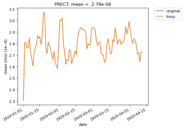
[38]:
# Time-series plot of PRECT mean in col_ds 'original' dataset - first 100 daysa
ldcpy.plot(
    col_prect,
    "PRECT",
    sets=["original", "lossy"],
    calc="mean",
    plot_type="time_series",
    start=0,
    end=100,
)
[42]:
# print statistics about 'original', 'lossy', and diff between the two datasets for TMQ at time slice 365
ldcpy.compare_stats(
    col_tmq.isel(time=365), "TMQ", ["original", "lossy"], aggregate_dims=["lat", "lon"]
)
Warning - this data does not conatin weights, so averages will be unweighted.
| original | lossy | |
|---|---|---|
| mean | 16.586 | 16.541 |
| variance | 239.68 | 238.4 |
| standard deviation | 15.482 | 15.44 |
| min value | 0.28534 | 0.28516 |
| min (abs) nonzero value | 0.28534 | 0.28516 |
| max value | 71.03 | 71 |
| probability positive | 0.50262 | 0.50262 |
| number of zeros | 0 | 0 |
| spatial autocorr - latitude | nan | nan |
| spatial autocorr - longitude | nan | nan |
| entropy estimate | 0.25738 | 0.092099 |
| lossy | |
|---|---|
| max abs diff | 0.0073329 |
| min abs diff | 0.0020776 |
| mean abs diff | 0.0047053 |
| mean squared diff | 2.2139e-05 |
| root mean squared diff | 0.0053893 |
| normalized root mean squared diff | 7.6178e-05 |
| normalized max pointwise error | 0.00010365 |
| pearson correlation coefficient | 0.99768 |
| ks p-value | nan |
| spatial relative error(% > 0.0001) | 0.52356 |
| max spatial relative error | 0.0077153 |
| DSSIM | nan |
The original data for FLNS and TMQ and TS and PRECT (from Amazon S3 in the “ncar-cesm-lens-baker-lossy-compression-test” bucket) was loaded above using method 1. An alternative would be to create our own catalog for this data for use with intake-esm. To illustrate this, we created a test_catalog.csv and test_collection.json file for this particular simple example.
We first open our collection.
[43]:
my_col_loc = "./collections/test_collection.json"
my_col = intake.open_esm_datastore(my_col_loc)
my_col
test catalog with 1 dataset(s) from 4 asset(s):
| unique | |
|---|---|
| component | 1 |
| frequency | 1 |
| experiment | 1 |
| variable | 4 |
| path | 4 |
| derived_variable | 0 |
[44]:
# printing the head() gives us the file names
my_col.df.head()
[44]:
| component | frequency | experiment | variable | path | |
|---|---|---|---|---|---|
| 0 | atm | daily | 20C | TS | s3://ncar-cesm-lens-baker-lossy-compression-te... |
| 1 | atm | daily | 20C | PRECT | s3://ncar-cesm-lens-baker-lossy-compression-te... |
| 2 | atm | daily | 20C | FLNS | s3://ncar-cesm-lens-baker-lossy-compression-te... |
| 3 | atm | daily | 20C | TMQ | s3://ncar-cesm-lens-baker-lossy-compression-te... |
Let’s load all of these into our dictionary! (So we don’t need to do the search to make a subset of variables as above in Method 2.)
[45]:
my_dset_dict = my_col.to_dataset_dict(
    zarr_kwargs={"consolidated": True, "decode_times": True},
    storage_options={"anon": True},
)
my_dset_dict
--> The keys in the returned dictionary of datasets are constructed as follows:
        'component.experiment.frequency'
[45]:
{'atm.20C.daily': <xarray.Dataset> Size: 28GB
 Dimensions:    (time: 31390, lat: 192, lon: 288, nbnd: 2)
 Coordinates:
   * lat        (lat) float64 2kB -90.0 -89.06 -88.12 -87.17 ... 88.12 89.06 90.0
   * lon        (lon) float64 2kB 0.0 1.25 2.5 3.75 ... 355.0 356.2 357.5 358.8
   * time       (time) object 251kB 1920-01-01 12:00:00 ... 2005-12-31 12:00:00
     time_bnds  (time, nbnd) object 502kB dask.array<chunksize=(15695, 2), meta=np.ndarray>
 Dimensions without coordinates: nbnd
 Data variables:
     FLNS       (time, lat, lon) float32 7GB dask.array<chunksize=(576, 192, 288), meta=np.ndarray>
     PRECT      (time, lat, lon) float32 7GB dask.array<chunksize=(576, 192, 288), meta=np.ndarray>
     TMQ        (time, lat, lon) float32 7GB dask.array<chunksize=(576, 192, 288), meta=np.ndarray>
     TS         (time, lat, lon) float32 7GB dask.array<chunksize=(576, 192, 288), meta=np.ndarray>
 Attributes: (12/16)
     Conventions:                     CF-1.0
     NCO:                             netCDF Operators version 4.7.9 (Homepage...
     Version:                         $Name$
     case:                            b.e11.B20TRC5CNBDRD.f09_g16.031
     host:                            ys0219
     initial_file:                    b.e11.B20TRC5CNBDRD.f09_g16.001.cam.i.19...
     ...                              ...
     topography_file:                 /glade/p/cesmdata/cseg/inputdata/atm/cam...
     intake_esm_attrs:component:      atm
     intake_esm_attrs:frequency:      daily
     intake_esm_attrs:experiment:     20C
     intake_esm_attrs:_data_format_:  zarr
     intake_esm_dataset_key:          atm.20C.daily}
[46]:
# we again just want the 20th century daily data
my_ds = my_dset_dict["atm.20C.daily"]
my_ds
[46]:
<xarray.Dataset> Size: 28GB
Dimensions:    (time: 31390, lat: 192, lon: 288, nbnd: 2)
Coordinates:
  * lat        (lat) float64 2kB -90.0 -89.06 -88.12 -87.17 ... 88.12 89.06 90.0
  * lon        (lon) float64 2kB 0.0 1.25 2.5 3.75 ... 355.0 356.2 357.5 358.8
  * time       (time) object 251kB 1920-01-01 12:00:00 ... 2005-12-31 12:00:00
    time_bnds  (time, nbnd) object 502kB dask.array<chunksize=(15695, 2), meta=np.ndarray>
Dimensions without coordinates: nbnd
Data variables:
    FLNS       (time, lat, lon) float32 7GB dask.array<chunksize=(576, 192, 288), meta=np.ndarray>
    PRECT      (time, lat, lon) float32 7GB dask.array<chunksize=(576, 192, 288), meta=np.ndarray>
    TMQ        (time, lat, lon) float32 7GB dask.array<chunksize=(576, 192, 288), meta=np.ndarray>
    TS         (time, lat, lon) float32 7GB dask.array<chunksize=(576, 192, 288), meta=np.ndarray>
Attributes: (12/16)
    Conventions:                     CF-1.0
    NCO:                             netCDF Operators version 4.7.9 (Homepage...
    Version:                         $Name$
    case:                            b.e11.B20TRC5CNBDRD.f09_g16.031
    host:                            ys0219
    initial_file:                    b.e11.B20TRC5CNBDRD.f09_g16.001.cam.i.19...
    ...                              ...
    topography_file:                 /glade/p/cesmdata/cseg/inputdata/atm/cam...
    intake_esm_attrs:component:      atm
    intake_esm_attrs:frequency:      daily
    intake_esm_attrs:experiment:     20C
    intake_esm_attrs:_data_format_:  zarr
intake_esm_dataset_key: atm.20C.dailyNow we can make a dataset for each variable as before.
[47]:
my_ts = my_ds["TS"].to_dataset()
my_tmq = my_ds["TMQ"].to_dataset()
my_prect = my_ds["PRECT"].to_dataset()
my_flns = my_ds["FLNS"].to_dataset()
And now we can form new collections as before and do comparisons…
[ ]:
[ ]: